Is it possible to reduce the sample size requirements of a stepped wedge cluster randomized trial simply by collecting baseline information? In a trial with randomization at the individual level, it is generally the case that if we are able to measure an outcome for subjects at two time periods, first at baseline and then at follow-up, we can reduce the overall sample size. But does this extend to (a) cluster randomized trials generally, and to (b) stepped wedge designs more specifically?
The answer to (a) is a definite “yes,” as described in a 2012 paper by Teerenstra et al (more details on that below). As for (b), two colleagues on the Design and Statistics Core of the NIA IMPACT Collaboratory, Monica Taljaard and Fan Li, and I have just started thinking about this. Ultimately, we hope to have an analytic solution that provides more formal guidance for stepped wedge designs; but to get things started, we thought we could explore a bit using simulation.
Quick overview
Generally speaking, why might baseline measurements have any impact at all? The curse of any clinical trial is variability - the more noise (variability) there is in the outcome, the more difficult it is to identify the signal (effect). For example, if we are interested in measuring the impact of an intervention on the quality of life (QOL) across a diverse range of patients, the measurement (which typically ranges from 0 to 1) might vary considerably from person to person, regardless of the intervention. If the intervention has a real but moderate effect of, say, 0.1 points, it could easily get lost if the standard deviation is considerably larger, say 0.25.
It turns out that if we collect baseline QOL scores and can “control” for those measurements in some way (by conducting a repeated measures analysis, using ANCOVA, or assessing the difference itself as an outcome), we might be able to reduce the variability across study subjects sufficiently to give us a better chance at picking up the signal. Previously, I’ve written about baseline covariate adjustment in the context of clinical trials where randomization is at the individual subject level; now we will turn to the case where randomization is at the cluster or site level.
This post focuses on work already done to derive design effects for parallel cluster randomized trials (CRTs) that collect baseline measurements; we will get to stepped wedge designs in future posts. I described the design effect pretty generally in an earlier post, but the paper by Teerenstra et al, titled “A simple sample size formula for analysis of covariance in cluster randomized trials” provides a great foundation to understand how baseline measurements can impact sample sizes in clustered designs.
Here’s a brief outline of what follows: after showing an example based on a simple 2-arm randomized control trial with 350 subjects that has 80% power to detect a standardized effect size of 0.3, I describe and simulate a series of designs with cluster sizes of 30 subjects that require progressively fewer clusters but also provide 80% power under the same effect size and total variance assumptions: a simple CRT that needs 64 sites, a cross-sectional pre-post design that needs 52, a repeated measures design that needs 38, and a repeated measures design that models follow-up outcomes only (i.e. uses an ANCOVA model) that requires only 32.
Simple RCT
We start with a simple RCT (without any clustering) that randomizes individuals to treatment or control.
\[ Y_{i} = \alpha + \delta Z_{i} + s_{i} \] where \(Y_{i}\) is a continuous outcome measure for individual \(i\), and \(Z_{i}\) is the treatment status of individual \(i\). \(\delta\) is the treatment effect. \(s_{i} \sim N(0, \sigma_s^2)\) are the individual random effects or noise.
Now that we are about to start coding, here are the necessary packages:
RNGkind("L'Ecuyer-CMRG")
set.seed(19287)

library(simstudy)
library(ggplot2)
library(lmerTest)
library(parallel)
library(data.table)
library(pwr)
library(gtsummary)
library(paletteer)
library(magrittr)
In the examples that follow, overall variance \(\sigma^2 = 64\). In this first example, then, \(\sigma_s^2 = 64\) since that is the only source of variation. The overall effect size \(\delta\), which is the difference in average scores across treatment groups, is assumed to be 2.4, a standardized effect size \(2.4/8 = 0.3.\) We will need to generate 350 individual subjects (175 in each arm) to achieve power of 80%.
pwr.t.test(d = 0.3, power = 0.80)##
## Two-sample t test power calculation
##
## n = 175
## d = 0.3
## sig.level = 0.05
## power = 0.8
## alternative = two.sided
##
## NOTE: n is number in *each* groupData generation process
Here is the data definition and generation process:
simple_rct <- function(N) {

  # data definition for outcome

  defS <- defData(varname = "rx", formula = "1;1", dist = "trtAssign")
  defS <- defData(defS, varname = "y", formula = "2.4*rx", variance = 64, dist = "normal")

  dd <- genData(N, defS)

  dd[]
}

dd <- simple_rct(350)
Here is a visualization of the outcome measures by treatment arm.
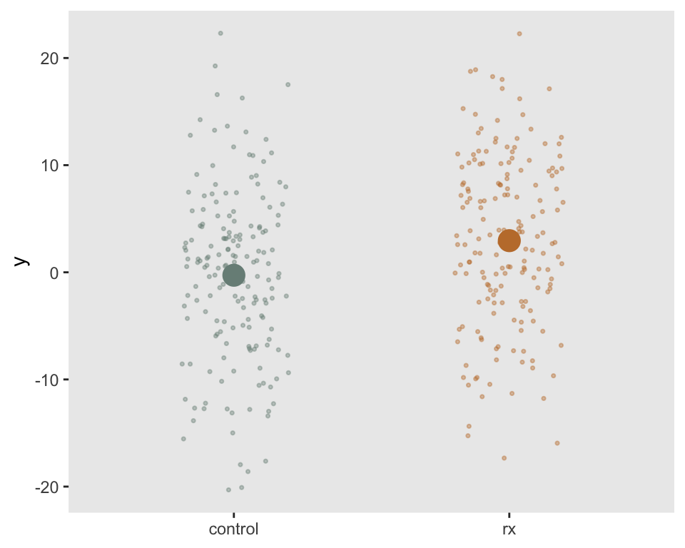
Estimating effect size
A simple linear regression model estimates the effect size:
fit1 <- lm(y ~  rx, data = dd)
tbl_regression(fit1) %>%
modify_footnote(ci ~ NA, abbreviation = TRUE)| Characteristic | Beta | 95% CI | p-value |
|---|---|---|---|
| rx | 3.2 | 1.6, 4.9 | <0.001 |
Confirming power
We can confirm the power by repeatedly generating data sets and fitting models, recording the p-values for each replication.
replicate <- function() {
  dd <- simple_rct(350)
  fit1 <- lm(y ~  rx, data = dd)

  coef(summary(fit1))["rx", "Pr(>|t|)"]
}

p_values <- mclapply(1:1000, function(x) replicate(), mc.cores = 4)
Here is the estimated power based on 1000 replications:
mean(unlist(p_values) < 0.05)## [1] 0.79Parallel cluster randomized trial
If we need to randomize at the site level (i.e., conduct a CRT), we can describe the data generation process as
\[Y_{ij} = \alpha + \delta Z_{j} + c_j + s_i\]
where \(Y_{ij}\) is a continuous outcome for subject \(i\) in site \(j\). \(Z_{j}\) is the treatment indicator for site \(j\). Again, \(\delta\) is the treatment effect. \(c_j \sim N(0,\sigma_c^2)\) is a site level effect, and \(s_i \sim N(0, \sigma_s^2)\) is the subject level effect. The correlation of any two subjects in a cluster is \(\rho\) (the ICC):
\[\rho = \frac{\sigma_c^2}{\sigma_c^2 + \sigma_s^2}\]
If we have a pre-specified number (\(n\)) of subjects at each site, we can estimate the sample size required in the CRT might applying a design effect \(1+(n-1)\rho\) to the sample size of an RCT that has the same overall variance. So, if \(\sigma_c^2 + \sigma_s^2 = 64\), we can augment the sample size we used in the initial example. If \(\sigma_c^2 = 9.6\) + \(\sigma_s^2 = 54.4\), \(\rho = 0.15\). We anticipate having 30 subjects at each site so the design effect is
\[1 + (30 - 1) \times 0.15 = 5.35\]
This means we will need \(5.35 \times 350 = 1872\) total subjects based on the same effect size and power assumptions. Since we anticipate 30 subjects per site, we need \(1872 / 30 = 62.4\) sites - we will round up to the nearest even number and use 64 sites.
Data generation process
simple_crt <- function(nsites, n) {

  defC <- defData(varname = "rx", formula = "1;1", dist = "trtAssign")
  defC <- defData(defC, varname = "c", formula = "0", variance = 9.6, dist = "normal")

  defS <- defDataAdd(varname="y", formula="c + 2.4*rx", variance = 54.4, dist="normal")

# site/cluster level data

  dc <- genData(nsites, defC, id = "site")

# individual level data

  dd <- genCluster(dc, "site", n, "id")
  dd <- addColumns(defS, dd)

  dd[]
}

dd <- simple_crt(20, 50)
Once again, the sites randomized to the treatment arm are colored red:
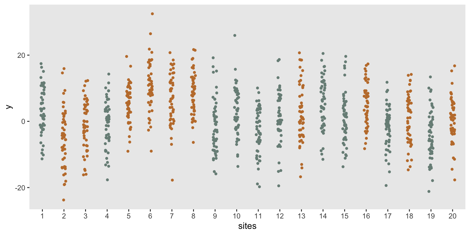
Estimating effect size
A mixed effects model is used to estimate the effect size. I’m using a larger data set to recover the parameters used in the data generation process:
dd <- simple_crt(200,100)

fit2 <- lmer(y ~  rx + (1|site), data = dd)
tbl_regression(fit2, tidy_fun = broom.mixed::tidy)  %>%
modify_footnote(ci ~ NA, abbreviation = TRUE)| Characteristic | Beta | 95% CI | p-value |
|---|---|---|---|
| rx | 1.2 | 0.21, 2.1 | 0.018 |
| site.sd__(Intercept) | 3.4 | ||
| Residual.sd__Observation | 7.4 |
Confirming power
Now, I will confirm power using 64 sites with 30 subjects per site, for a total of 1920 subjects (compared with only 350 in the RCT):
replicate <- function() {
  dd <- simple_crt(64, 30)
  fit2 <- lmer(y ~  rx + (1|site), data = dd)

  coef(summary(fit2))["rx", "Pr(>|t|)"]
}

p_values <- mclapply(1:1000, function(x) replicate(), mc.cores = 4)

mean(unlist(p_values) < 0.05)
## [1] 0.8CRT with baseline measurement
We paid quite a hefty price moving from an RCT to a CRT in terms of the number of subjects we need to collect data on. If these data are coming from administrative systems, that added burden might not be an issue, but if we need to consent all the subjects and survey them individually, this could be quite burdensome.
We may be able to decrease the required number of clusters (i.e. reduce the design effect) if we can collect baseline measurements of the outcome. The baseline and follow-up measurements can be collected from the same subjects or different subjects, though the impact on the design effect depends on what approach is taken.
\[ Y_{ijk} = \alpha_0 + \alpha_1 k + \delta_{0} Z_j + \delta_{1}k Z_{j} + c_j + cp_{jk} + s_{ij} + sp_{ijk} \]
where \(Y_{ijk}\) is a continuous outcome measure for individual \(i\) in site \(j\) and measurement \(k \in \{0,1\}\). \(k=0\) for baseline measurement, and \(k=1\) for the follow-up. \(Z_{j}\) is the treatment status of cluster \(j\), \(Z_{j} \in \{0,1\}.\) \(\alpha_0\) is the mean outcome at baseline for subjects in the control clusters, \(\alpha_1\) is the change from baseline to follow-up in the control arm, \(\delta_{0}\) is the difference at baseline between control and treatment arms (we would expect this to be \(0\) in a randomized trial), and \(\delta_{1}\) is the difference in the change from baseline to follow-up between the two arms. (In a randomized trial, since \(\delta_0\) should be close to \(0\), \(\delta_1\) is the treatment effect.)
The model has cluster-specific and subject-specific random effects. For both, there can be time-invariant effects and time-varying effects. \(c_j \sim N(0,\sigma_c^2)\) are time invariant site-specific effects, and \(cp_{jk}\) are the site-specific period (time varying) effects, where \(c_{jk} \sim N(0, \sigma_{cp}^2)\). At the subject level there can be \(s_{ij} \sim N(0, \sigma_s^2)\) and \(sp_{ijk} \sim N(0, \sigma_{sp}^2)\).
Here is the generic code that will facilitate data generation in this model:
crt_base <- function(effect, nsites, n, s_c, s_cp, s_s, s_sp) {

  defC <- defData(varname = "c", formula = 0, variance = "..s_c")
  defC <- defData(defC, varname = "rx", formula = "1;1", dist = "trtAssign")

  defCP <- defDataAdd(varname = "c.p", formula = 0, variance = "..s_cp")

  defS <- defDataAdd(varname = "s", formula = 0, variance = "..s_s")

  defSP <- defDataAdd(varname = "y",
    formula = "..effect * rx * period + c + c.p + s",
    variance ="..s_sp")

  dc <- genData(nsites, defC, id = "site")

  dcp <- addPeriods(dc, 2, "site")
  dcp <- addColumns(defCP, dcp)
  dcp <- dcp[, .(site, period, c.p, timeID)]

  ds <- genCluster(dc, "site", n, "id")
  ds <- addColumns(defS, ds)

  dsp <- addPeriods(ds, 2)
  setnames(dsp, "timeID", "obsID")

  setkey(dsp, site, period)
  setkey(dcp, site, period)

  dd <- merge(dsp, dcp)
  dd <- addColumns(defSP, dd)
  setkey(dd, site, id, period)

  dd[]
}
Design effect
In their paper, Teerenstra et al develop a design effect that takes into account the baseline measurement. Here are a few key quantities that are needed for the calculation:
The correlation of two subject measurements in the same cluster and same time period is the ICC or \(\rho\), and is:
\[\rho = \frac{\sigma_c^2 + \sigma_{cp}^2}{\sigma_c^2 + \sigma_{cp}^2 + \sigma_s^2 + \sigma_{sp}^2} \]
In order to estimate design effect, we need two more correlations. The correlation between baseline and follow-up random effects at the cluster level is
\[\rho_c = \frac{\sigma_c^2}{\sigma_c^2 + \sigma_{cp}^2}\]
and the correlation between baseline and follow-up random effects at the subject level is
\[\rho_s = \frac{\sigma_s^2}{\sigma_s^2 + \sigma_{sp}^2}\]
A value \(r\) is used to estimate the design effect, and is defined as
\[ r = \frac{n\rho\rho_c + (1-\rho)\rho_s}{1 + (n-1)\rho}\]
If we are able to collect baseline measurements and our focus is on estimating \(\delta_1\) from the model, the design effect is slightly modified from before:
\[ (1 + (n-1)\rho)(2(1-r)) \]
Cross-sectional cohorts
We may not be able to collect two measurements for each subject at a site, but if we can collect measurements on two different cohorts, one at baseline before the intervention is implemented, and one cohort in a second period (either after the intervention has been implemented or not, depending on the randomization assignment of the cluster), we might be able to reduce the number of clusters.
In this case, \(\sigma_s^2 = 0\) and \(\rho_s = 0\), so the general model reduces to
\[ Y_{ijk} = \alpha_0 + \alpha_1 k + \delta_{0} Z_j + \delta_{1} k Z_{j} + c_j + cp_{jk} + sp_{ijk} \]
Data generation process
The parameters for this simulation are \(\delta_1 = 2.4\), \(\sigma_c^2 = 6.8\), \(\sigma_{cp}^2 = 2.8\), \(\sigma_{sp}^2 = 54.4\). Total variance \(\sigma_c^2 + \sigma_{cp}^2 + \sigma_{sp}^2 = 6.8 + 2.8 + 54.4 = 64\), as used previously.
dd <- crt_base(effect = 2.4, nsites = 20, n = 30, s_c=6.8, s_cp=2.8, s_s=0, s_sp=54.4)Here is a visualization of the outcome measures by site and by period, with the sites in the treatment arm colored in red (only in the follow-up period).
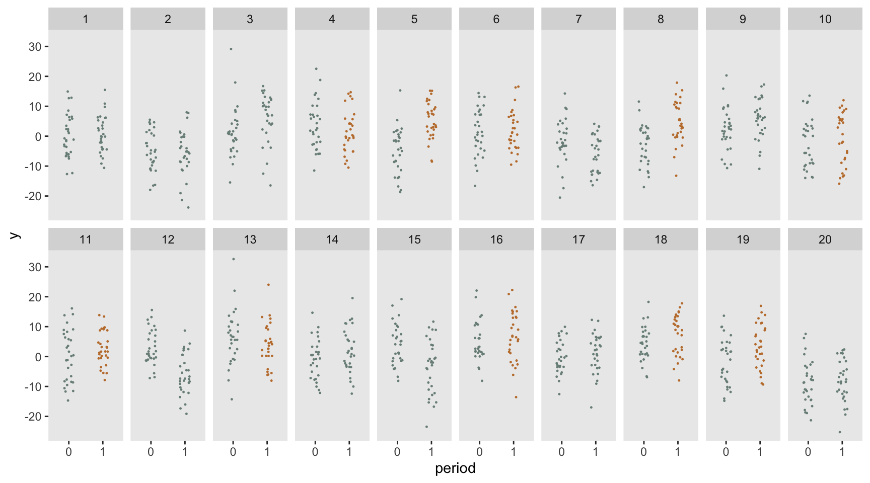
Estimating effect size
To estimate the effect size we fit a mixed effect model with cluster-specific effects only (both time invariant and time varying).
dd <- crt_base(effect = 2.4, nsites = 200, n = 100, s_c=6.8, s_cp=2.8, s_s=0, s_sp=54.4)

fit3 <- lmer(y ~ period*rx+ (1|timeID:site) + (1 | site), data = dd)
tbl_regression(fit3, tidy_fun = broom.mixed::tidy)  %>%
modify_footnote(ci ~ NA, abbreviation = TRUE)| Characteristic | Beta | 95% CI | p-value |
|---|---|---|---|
| period | -0.03 | -0.52, 0.46 | >0.9 |
| rx | 0.17 | -0.78, 1.1 | 0.7 |
| period * rx | 2.7 | 2.0, 3.4 | <0.001 |
| timeID:site.sd__(Intercept) | 1.6 | ||
| site.sd__(Intercept) | 2.9 | ||
| Residual.sd__Observation | 7.4 |
Confirming power
Based on the variance assumptions, we can update our design effect:
s_c <- 6.8
s_cp <- 2.8
s_s <- 0
s_sp <- 54.4

rho <- (s_c + s_cp)/(s_c + s_cp + s_s + s_sp)
rho_c <- s_c/(s_c + s_cp)
rho_s <- s_s/(s_s + s_sp)

n <- 30

r <- (n * rho * rho_c + (1-rho) * rho_s) / (1 + (n-1) * rho)
The design effect for the CRT without any baseline measurement was 5.35. With the two-cohort design, the design effect is reduced slightly:
(des_effect <- (1 + (n - 1) * rho) * 2 * (1 - r))## [1] 4.3des_effect * 350 / n## [1] 50The desired number of sites is over 50, so rounding up to the next even number gives us 52:
replicate <- function() {
  dd <- crt_base(2.4, 52, 30, s_c = 6.8, s_cp = 2.8, s_s = 0, s_sp = 54.4)
  fit3 <- lmer(y ~ period * rx+ (1|timeID:site) + (1 | site), data = dd)

  coef(summary(fit3))["period:rx", "Pr(>|t|)"]
}

p_values <- mclapply(1:1000, function(x) replicate(), mc.cores = 4)

mean(unlist(p_values) < 0.05)
## [1] 0.8Repeated measurements
We can reduce the number of clusters further if instead of measuring one cohort prior to the intervention and another after the intervention, we measure a single cohort twice - once at baseline and once at follow-up. Now we use the full model that decomposes the subject level variance into a time invariant effect (\(c_j\)) and a time varying effect \(cp_{jk}\):
\[ Y_{ijk} = \alpha_0 + \alpha_1 k + \delta_{0} Z_j + \delta_{1} k Z_{j} + c_j + cp_{jk} + s_{ij} + sp_{ijk} \]
Data generation process
These are the parameters, \(\delta_1 = 2.4\), \(\sigma_c^2 = 6.8\), \(\sigma_{cp}^2 = 2.8\), \(\sigma_s = 38,\) and \(\sigma_{sp}^2 = 16.4\).
dd <- crt_base(effect=2.4, nsites=20, n=30, s_c=6.8, s_cp=2.8, s_s=38, s_sp=16.4)Here is what the data look like; each line represents an individual subject at the two time points, baseline and follow-up.
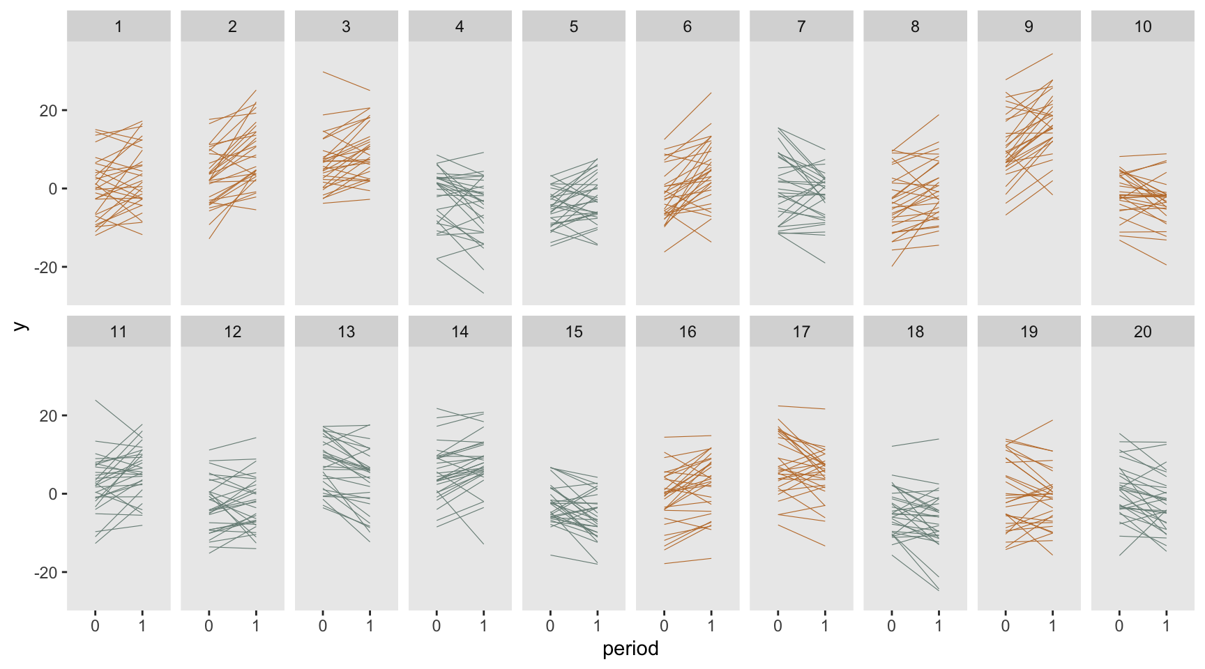
Estimating effect size
The mixed effect model includes cluster-specific effects only (both time invariant and time varying), as well as subject level effects. Again, total variance (\(\sigma_c^2 + \sigma_{cp}^2 + \sigma_s^2 + \sigma_{sp}^2\)) is 64.
dd <- crt_base(effect = 2.4, nsites = 200, n = 100,
  s_c = 6.8, s_cp = 2.8, s_s = 38, s_sp = 16.4)

fit4 <- lmer(y ~ period*rx + (1 | id:site) + (1|timeID:site) + (1 | site), data = dd)
tbl_regression(fit4, tidy_fun = broom.mixed::tidy)  %>%
modify_footnote(ci ~ NA, abbreviation = TRUE)| Characteristic | Beta | 95% CI | p-value |
|---|---|---|---|
| period | -0.21 | -0.73, 0.31 | 0.4 |
| rx | -0.19 | -1.1, 0.73 | 0.7 |
| period * rx | 2.4 | 1.7, 3.2 | <0.001 |
| id:site.sd__(Intercept) | 6.2 | ||
| timeID:site.sd__(Intercept) | 1.8 | ||
| site.sd__(Intercept) | 2.7 | ||
| Residual.sd__Observation | 4.1 |
Confirming power
Based on the variance assumptions, we can update our design effect a second time:
s_c <- 6.8
s_cp <- 2.8
s_s <- 38
s_sp <- 16.4

rho <- (s_c + s_cp)/(s_c + s_cp + s_s + s_sp)
rho_c <- s_c/(s_c + s_cp)
rho_s <- s_s/(s_s + s_sp)

n <- 30

r <- (n * rho * rho_c + (1-rho) * rho_s) / (1 + (n-1) * rho)
And again, the design effect (and sample size requirement) is reduced:
(des_effect <- (1 + (n - 1) * rho) * 2 * (1 - r))## [1] 3.1des_effect * 350 / n## [1] 37The desired number of sites is over 36, so I will round up to 38:
replicate <- function() {
  dd <- crt_base(2.4, 38, 30, s_c = 6.8, s_cp = 2.8, s_s = 38, s_sp = 16.4)
  fit4 <-  lmer(y ~ period*rx + (1 | id:site) + (1|timeID:site) + (1 | site), data = dd)

  coef(summary(fit4))["period:rx", "Pr(>|t|)"]
}

p_values <- mclapply(1:1000, function(x) replicate(), mc.cores = 4)

mean(unlist(p_values) < 0.05)
## [1] 0.79Repeated measurements - ANCOVA
We may be able to reduce the number of clusters even further by changing the model so that we are comparing follow-up outcomes of the two treatment arms (as opposed to measuring the differences in changes as we just did). This model is
\[ Y_{ij1} = \alpha_0 + \gamma Y_{ij0} + \delta Z_j + c_j + s_{ij} \]
where we have adjusted for baseline measurement \(Y_{ij0}.\) Even though the estimation model has changed, I am using the exact same data generation process as before, with the same effect size and variance assumptions:
dd <- crt_base(effect = 2.4, nsites = 200, n = 100,
  s_c = 6.8, s_cp = 2.8, s_s = 38, s_sp = 16.4)

dobs <- dd[, .(site, rx, id, period, timeID, y)]
dobs <- dcast(dobs, site + rx + id ~ period, value.var = "y")

fit5 <- lmer(`1` ~ `0` + rx + (1 | site), data = dobs)
tbl_regression(fit5, tidy_fun = broom.mixed::tidy)  %>%
modify_footnote(ci ~ NA, abbreviation = TRUE)| Characteristic | Beta | 95% CI | p-value |
|---|---|---|---|
| 0 | 0.70 | 0.69, 0.71 | <0.001 |
| rx | 2.5 | 1.8, 3.1 | <0.001 |
| site.sd__(Intercept) | 2.2 | ||
| Residual.sd__Observation | 5.3 |
Design effect
Teerenstra et al derived an alternative design effect that is specific to the ANCOVA model:
\[ (1 + (n-1)\rho) (1-r^2) \]
where \(r\) is the same as before. Since \((1-r^2) < 2(1-r), \ 0 \le r < 1\), this will be a reduction from the earlier model.
(des_effect <- (1 + (n - 1) * rho) * (1 - r^2))## [1] 2.7des_effect * 350 / n## [1] 31Confirming power
replicate <- function() {

  dd <- crt_base(2.4, 32, 30, s_c = 6.8, s_cp = 2.8, s_s = 38, s_sp = 16.4)
  dobs <- dd[, .(site, rx, id, period, timeID, y)]
  dobs <- dcast(dobs, site + rx + id ~ period, value.var = "y")

  fit5 <- lmer(`1` ~ `0` + rx + (1 | site), data = dobs)
  coef(summary(fit5))["rx", "Pr(>|t|)"]
}

p_values <- mclapply(1:1000, function(x) replicate(), mc.cores = 4)

mean(unlist(p_values) < 0.05)
## [1] 0.78Next steps
These simulations confirmed the design effects derived by Teerenstra et al. In the next post, we will turn to baseline measurements in the context of a stepped wedge design, to see if these results translate to a more complex setting. The design effects themselves have not yet been derived. In the meantime, to get yourself psyched up for what is coming, you can read more generally about stepped wedge designs here, here, here, here, here, and here.
Update: you can now proceed directly to the second part.
Reference:
Teerenstra, Steven, Sandra Eldridge, Maud Graff, Esther de Hoop, and George F. Borm. “A simple sample size formula for analysis of covariance in cluster randomized trials.” Statistics in medicine 31, no. 20 (2012): 2169-2178.
Support:
This work was supported in part by the National Institute on Aging (NIA) of the National Institutes of Health under Award Number U54AG063546, which funds the NIA IMbedded Pragmatic Alzheimer’s Disease and AD-Related Dementias Clinical Trials Collaboratory (NIA IMPACT Collaboratory). The author, a member of the Design and Statistics Core, was the sole writer of this blog post and has no conflicts. The content is solely the responsibility of the author and does not necessarily represent the official views of the National Institutes of Health.