In the last two posts, I introduced the notion of time-varying intra-cluster correlations in the context of stepped-wedge study designs. (See here and here). Though I generated lots of data for those posts, I didn’t fit any models to see if I could recover the estimates and any underlying assumptions. That’s what I am doing now.
My focus here is on the simplest case, where the ICC’s are constant over time and between time. Typically, I would just use a mixed-effects model to estimate the treatment effect and account for variability across clusters, which is easily done in R using the lme4 package; if the outcome is continuous the function lmer is appropriate. I thought, however, it would also be interesting to use the rstan package to fit a Bayesian hierarchical model.
While it is always fun to explore new methods, I have a better justification for trying this approach: as far as I can tell, lme4 (or nlme for that matter) cannot handle the cases with more complex patterns of between-period intra-cluster correlation that I focused on last time. A Bayesian hierarchical model should be up to the challenge. I thought that it would be best to start with a simple case before proceeding to the situation where I have no clear option in R. I’ll do that next time.
Data generation
I know I am repeating myself a little bit, but it is important to be clear about the data generation process that I am talking about here.
\[Y_{ic} = \mu + \beta_1X_{c} + b_c + e_{ic},\]
where \(Y_{ic}\) is a continuous outcome for subject \(i\) in cluster \(c\), and \(X_c\) is a treatment indicator for cluster \(c\) (either 0 or 1). The underlying structural parameters are \(\mu\), the grand mean, and \(\beta_1\), the treatment effect. The unobserved random effects are, \(b_c \sim N(0, \sigma^2_b)\), the normally distributed group level effect, and \(e_{ic} \sim N(0, \sigma^2_e)\), the normally distributed individual-level effect.
library(simstudy)

defc <- defData( varname = "ceffect", formula = 0.0, variance = 0.15,
                 dist = "normal", id = "cluster")
defc <- defData(defc, varname = "m", formula = 15, dist = "nonrandom")

defa <- defDataAdd(varname = "Y",
                   formula = "0 + 0.10  * period + 1 * rx + ceffect",
                   variance = 2, dist = "normal")

genDD <- function(defc, defa, nclust, nperiods, waves, len, start) {
  dc <- genData(nclust, defc)
  dp <- addPeriods(dc, nperiods, "cluster")
  dp <- trtStepWedge(dp, "cluster", nWaves = waves, lenWaves = len,
                     startPer = start)

  dd <- genCluster(dp, cLevelVar = "timeID", numIndsVar = "m",
                   level1ID = "id")
  dd <- addColumns(defa, dd)
  dd[]
}

set.seed(2822)
dx <- genDD(defc, defa, 60, 7, 4, 1, 2)

dx
## cluster period ceffect m timeID startTrt rx id Y
## 1: 1 0 -0.05348668 15 1 2 0 1 -0.1369149
## 2: 1 0 -0.05348668 15 1 2 0 2 -1.0030891
## 3: 1 0 -0.05348668 15 1 2 0 3 3.1169339
## 4: 1 0 -0.05348668 15 1 2 0 4 -0.8109585
## 5: 1 0 -0.05348668 15 1 2 0 5 0.2285751
## ---
## 6296: 60 6 0.10844859 15 420 5 1 6296 0.4171770
## 6297: 60 6 0.10844859 15 420 5 1 6297 1.5127632
## 6298: 60 6 0.10844859 15 420 5 1 6298 0.5194967
## 6299: 60 6 0.10844859 15 420 5 1 6299 -0.3120285
## 6300: 60 6 0.10844859 15 420 5 1 6300 2.0493244Using lmer to estimate treatment effect and ICC’s
As I derived earlier, the within- and between-period ICC’s under this data generating process are:
\[ICC = \frac{\sigma^2_b}{\sigma^2_b + \sigma^2_e}\]
Using a linear mixed-effects regression model we can estimate the fixed effects (the time trend and the treatment effect) as well as the random effects (cluster- and individual-level variation, \(\sigma^2_b\) and \(\sigma^2_e\)). The constant ICC can be estimated directly from the variance estimates.
library(lme4)
library(sjPlot)

lmerfit <- lmer(Y ~ period + rx + (1 | cluster) , data = dx)

tab_model(lmerfit, show.icc = FALSE, show.dev = FALSE,
          show.p = FALSE, show.r2 = FALSE,
title = "Linear mixed-effects model")| Y | ||
|---|---|---|
| Predictors | Estimates | CI |
| (Intercept) | 0.09 | -0.03 – 0.21 |
| period | 0.08 | 0.05 – 0.11 |
| rx | 1.03 | 0.90 – 1.17 |
| Random Effects | ||
| σ2 | 2.07 | |
| τ00 cluster | 0.15 | |
| N cluster | 60 | |
| Observations | 6300 | |
Not surprisingly, this model recovers the parameters used in the data generation process. Here is the ICC estimate based on this sample:
(vars <- as.data.frame(VarCorr(lmerfit))$vcov)## [1] 0.1540414 2.0691434(iccest <- round(vars[1]/(sum(vars)), 3))## [1] 0.069Bayesian hierarchical model
To estimate the same model using Bayesian methods, I’m turning to rstan. If Bayesian methods are completely foreign to you or you haven’t used rstan before, there are obviously incredible resources out on the internet and in bookstores. (See here, for example.) While I have done some Bayesian modeling in the past and have read some excellent books on the topic (including Statistical Rethinking and Doing Bayesian Data Analysis, though I have not read Bayesian Data Analysis and I know I should.)
To put things simplistically, the goal of this method is to generate a posterior distribution \(P(\theta | observed \ data)\), where \(\theta\) is a vector of model parameters of interest. The Bayes theorem provides the underlying machinery for all of this to happen:
\[P(\theta | observed \ data) = \frac{P(observed \ data | \theta)}{P(observed \ data)} P(\theta)\] \(P(observed \ data | \theta)\) is the data likelihood and \(P(\theta)\) is the prior distribution. Both need to be specified in order to generate the desired posterior distribution. The general (again, highly simplistic) idea is that draws of \(\theta\) are repeatedly made from the prior distribution, and each time the likelihood is estimated which updates the probability of \(\theta\). At the completion of the iterations, we are left with a posterior distribution of \(\theta\) (conditional on the observed data).
This is my first time working with Stan, so it is a bit of an experiment. While things have worked out quite well in this case, I may be doing things in an unconventional (i.e. not quite correct) way, so treat this as more conceptual than tutorial - though it’ll certainly get you started.
Defining the model
In Stan, the model is specified in a separate stan program that is written using the Stan probabilistic programming language. The code can be saved as an external file and referenced when you want to sample data from the posterior distribution. In this case, I’ve save the following code in a file named nested.stan.
This stan file includes at least 3 “blocks”: data, parameters, and model. The data block defines the data that will be provided by the user, which includes the outcome and predictor data, as well as other information required for model estimation. The data are passed from R using a list.
The parameters of the model are defined explicitly in the parameter block; in this case, we have regression parameters, random effects, and variance parameters. The transformed parameter block provides the opportunity to create parameters that depend on data and pre-defined parameters. They have no prior distributions per se, but can be used to simplify model block statements, or perhaps make the model estimation more efficient.
Since this is a Bayesian model, each of the parameters will have a prior distribution that can be specified in the model block; if there is no explicit specification of a prior for a parameter, Stan will use a default (non- or minimally-informative) prior distribution. The outcome model is also defined here.
There is also the interesting possibility of defining derived values in a block called generated quantities. These quantities will be functions of previously defined parameters and data. In this case, we might be interested in estimating the ICC along with an uncertainty interval; since the ICC is a function of cluster- and individual-level variation, we can derive and ICC estimate for each of the iterations. At the end of the sequence of iterations, we will have a posterior distribution of the ICC.
Here is the nested.stan file used for this analysis:
data {

  int<lower=0> N;              // number of individuals
  int<lower=1> K;              // number of predictors
  int<lower=1> J;              // number of clusters
  int<lower=1,upper=J> jj[N];  // group for individual
  matrix[N, K] x;              // predictor matrix
  vector[N] y;                 // outcome vector

}

parameters {

  vector[K] beta;           // intercept, time trend, rx effect
  real<lower=0> sigmalev1;  // cluster level standard deviation
  real<lower=0> sigma;      // individual level sd
  vector[J] ran;            // cluster level effects

}

transformed parameters{

  vector[N] yhat;

  for (i in 1:N)
    yhat[i] = x[i]*beta + ran[jj[i]];

}

model {
  ran ~ normal(0, sigmalev1);
  y ~ normal(yhat, sigma);
}

generated quantities {

  real<lower=0> sigma2;
  real<lower=0> sigmalev12;
  real<lower=0> icc;

  sigma2 = pow(sigma, 2);
  sigmalev12 = pow(sigmalev1, 2);
  icc = sigmalev12/(sigmalev12 + sigma2);

}
Estimating the model
Once the definition has been created, the next steps are to create the data set (as an R list) and call the functions to run the MCMC algorithm. The first function (stanc) converts the .stan file into C++ code. The function stan_model converts the C++ code into a stanmodel object. And the function sampling draws samples from the stanmodel object created in the second step.
library(rstan)
options(mc.cores = parallel::detectCores())

x <- as.matrix(dx[ ,.(1, period, rx)])
K <- ncol(x)
N <- dx[, length(unique(id))]
J <- dx[, length(unique(cluster))]
jj <- dx[, cluster]
y <- dx[, Y]

testdat <- list(N, K, J, jj, x, y)

rt <- stanc("Working/stan_icc/nested.stan")
sm <- stan_model(stanc_ret = rt, verbose=FALSE)
fit <- sampling(sm, data=testdat, seed = 3327, iter = 5000, warmup = 1000)
Looking at the diagnostics
Once the posterior distribution has been generated, it is important to investigate to see how well-behaved the algorithm performed. One way to do this is look at a series of trace plots that provide insight into how stable the algorithm was as it moved around the parameter space. In this example, I used 5000 draws but threw out the first 1000. Typically, the early draws show much more variability, so it is usual to ignore the “burn-in” phase when analyzing the posterior distribution.
The process didn’t actually generate 5000 draws, but rather 20,000. The process was simultaneously run four separate times. The idea is if things are behaving well, the parallel processes (called chains) should mix quite well - it should be difficult to distinguish between the chains. In the plot below each chain is represented by a different color.
I think it is prudent to ensure that all parameters behaved reasonably, but here I am providing trace plots to the variance estimates, the effect size estimate, and the ICC.
library(ggthemes)

pname <- c("sigma2", "sigmalev12", "beta[3]", "icc")
muc <- rstan::extract(fit, pars=pname,  permuted=FALSE, inc_warmup=FALSE)
mdf <- data.table(melt(muc))
mdf[parameters == "beta[3]", parameters := "beta[3] (rx effect)"]

ggplot(mdf,aes(x=iterations, y=value, color=chains)) +
  geom_line() +
  facet_wrap(~parameters, scales = "free_y") +
  theme(legend.position = "none",
        panel.grid = element_blank()) +
  scale_color_ptol()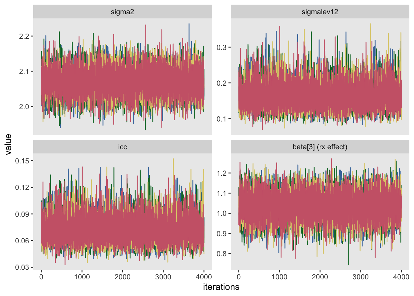
Evaluating the posterior distribution
Since these trace plots look fairly stable, it is reasonable to look at the posterior distribution. A summary of the distribution reports the means and percentiles for the parameters of interest. I am reprinting the results from lmer so you can see that the Bayesian estimates are pretty much identical to the mixed-effect model:
print(fit, pars=c("beta", "sigma2", "sigmalev12", "icc"))## Inference for Stan model: nested.
## 4 chains, each with iter=5000; warmup=1000; thin=1;
## post-warmup draws per chain=4000, total post-warmup draws=16000.
##
## mean se_mean sd 2.5% 25% 50% 75% 97.5% n_eff Rhat
## beta[1] 0.09 0 0.06 -0.03 0.05 0.09 0.13 0.21 3106 1
## beta[2] 0.08 0 0.02 0.05 0.07 0.08 0.09 0.11 9548 1
## beta[3] 1.03 0 0.07 0.90 0.99 1.03 1.08 1.16 9556 1
## sigma2 2.07 0 0.04 2.00 2.05 2.07 2.10 2.14 24941 1
## sigmalev12 0.16 0 0.03 0.11 0.14 0.16 0.18 0.24 13530 1
## icc 0.07 0 0.01 0.05 0.06 0.07 0.08 0.11 13604 1
##
## Samples were drawn using NUTS(diag_e) at Wed Jun 26 16:18:31 2019.
## For each parameter, n_eff is a crude measure of effective sample size,
## and Rhat is the potential scale reduction factor on split chains (at
## convergence, Rhat=1).| Y | ||
|---|---|---|
| Predictors | Estimates | CI |
| (Intercept) | 0.09 | -0.03 – 0.21 |
| period | 0.08 | 0.05 – 0.11 |
| rx | 1.03 | 0.90 – 1.17 |
| Random Effects | ||
| σ2 | 2.07 | |
| τ00 cluster | 0.15 | |
| N cluster | 60 | |
| Observations | 6300 | |
The ability to produce a density plot that shows the posterior distribution of the ICC is a pretty compelling reason to use Bayesian methods. The density plot provides an quick way to assess uncertainty of estimates for parameters that might not even be directly included in a linear mixed-effects model:
plot_dens <- function(fit, pars, p = c(0.05, 0.95),
                      fill = "grey80", xlab = NULL) {

  qs <- quantile(extract(fit, pars = pars)[[1]], probs = p)

  x.dens <- density(extract(fit, pars = pars)[[1]])
  df.dens <- data.frame(x = x.dens$x, y = x.dens$y)

  p <- stan_dens(fit, pars = c(pars), fill = fill, alpha = .1) +
    geom_area(data = subset(df.dens, x >= qs[1] & x <= qs[2]),
              aes(x=x,y=y), fill = fill, alpha = .4)

  if (is.null(xlab)) return(p)
  else return(p + xlab(xlab))
}

plot_dens(fit, "icc", fill = "#a1be97")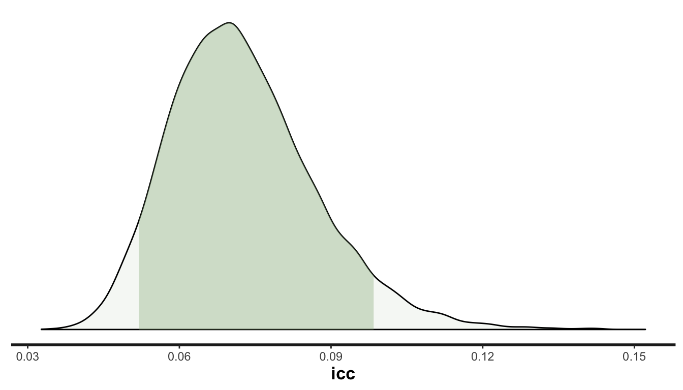
Next time, I will expand the stan model to generate parameter estimates for cases where the within-period and between-period ICC’s are not necessarily constant. I will also explore how we compare models in the context of Bayesian models, because we won’t always know the underlying data generating process!