Bayes models for estimation in stepped-wedge trials with non-trivial ICC patterns

Data generation

The data generating model this time around is only subtly different from before, but that difference is quite important. Rather than a single cluster-specific effect \(b_c\), there is now a vector of cluster effects \(\mathbf{b_c} = \left( b_{c1}, b_{c2}, \ldots, b_{cT} \right)\), where \(b_c \sim MVN(\mathbf{0}, \sigma^2 \mathbf{R})\) (see this earlier post for a description of the correlation matrix \(\mathbf{R}\).)

\[ Y_{ict} = \mu + \beta_0t + \beta_1X_{ct} + b_{ct} + e_{ict} \]

By altering the correlation structure of \(\mathbf{b_c}\) (that is \(\mathbf{R}\)), we can the change the structure of the ICC’s. (The data generation was the focus of the first two posts of this series, here and here. The data generating function genDD includes an argument where you can specify the two correlation structures, exchangeable and auto-regressive:

library(simstudy)

defc <- defData(varname = "mu", formula = 0, 
                dist = "nonrandom", id = "cluster")
defc <- defData(defc, "s2", formula = 0.15, dist = "nonrandom")
defc <- defData(defc, "m", formula = 15, dist = "nonrandom")

defa <- defDataAdd(varname = "Y", 
                   formula = "0 + 0.10  * period + 1 * rx + cteffect", 
                   variance = 2, dist = "normal")

genDD <- function(defc, defa, nclust, nperiods, 
                  waves, len, start, rho, corstr) {
  
  dc <- genData(nclust, defc)
  dp <- addPeriods(dc, nperiods, "cluster")
  dp <- trtStepWedge(dp, "cluster", nWaves = waves, lenWaves = len, 
                     startPer = start)
  dp <- addCorGen(dtOld = dp, nvars = nperiods, idvar = "cluster", 
                  rho = rho, corstr = corstr, dist = "normal", 
                  param1 = "mu", param2 = "s2", cnames = "cteffect")
  
  dd <- genCluster(dp, cLevelVar = "timeID", numIndsVar = "m", 
                   level1ID = "id")
  dd <- addColumns(defa, dd)
  dd[]
}

Constant between-period ICC’s

In this first scenario, the assumption is that the within-period ICC’s are larger than the between-period ICC’s and the between-period ICC’s are constant. This can be generated with random effects that have a correlation matrix with compound symmetry (or is exchangeable). In this case, we will have 60 clusters and 7 time periods:

set.seed(4119)
dcs <- genDD(defc, defa, 60, 7, 4, 1, 2, 0.6, "cs")

# correlation of "unobserved" random effects

round(cor(dcast(dcs[, .SD[1], keyby = .(cluster, period)], 
  formula = cluster ~ period, value.var = "cteffect")[, 2:7]), 2)

##      0    1    2    3    4    5
## 0 1.00 0.60 0.49 0.60 0.60 0.51
## 1 0.60 1.00 0.68 0.64 0.62 0.64
## 2 0.49 0.68 1.00 0.58 0.54 0.62
## 3 0.60 0.64 0.58 1.00 0.63 0.66
## 4 0.60 0.62 0.54 0.63 1.00 0.63
## 5 0.51 0.64 0.62 0.66 0.63 1.00

library(lme4)

lmerfit <- lmer(Y ~ period + rx + (1 | cluster/period) , data = dcs)
as.data.table(VarCorr(lmerfit))

##               grp        var1 var2       vcov     sdcor
## 1: period:cluster (Intercept) <NA> 0.05827349 0.2413990
## 2:        cluster (Intercept) <NA> 0.07816476 0.2795796
## 3:       Residual        <NA> <NA> 2.02075355 1.4215321

vs <- as.data.table(VarCorr(lmerfit))$vcov
vs[2]/sum(vs[1:2])  

## [1] 0.5728948

sum(vs[1:2])/sum(vs)

## [1] 0.06324808

vs[2]/sum(vs)          

## [1] 0.0362345

data {
  int<lower=0> N;              // number of unique individuals
  int<lower=1> K;              // number of predictors
  int<lower=1> J;              // number of clusters
  int<lower=0> T;              // number of periods
  int<lower=1,upper=J> jj[N];  // group for individual
  int<lower=1> tt[N];          // period for individual
  matrix[N, K] x;              // matrix of predctors
  vector[N] y;                 // matrix of outcomes
}

parameters {
  vector[K] beta;              // model fixed effects
  real<lower=0> sigmalev1;     // cluster variance (sd)
  real<lower=-1,upper=1> rho;  // correlation
  real<lower=0> sigma;         // individual level varianc (sd)
  
  matrix[J, T] ran;            // site level random effects (by period)
}
 
transformed parameters{ 
  
  cov_matrix[T] Sigma;
  vector[N] yhat;
  vector[T] mu0;
  
  for (t in 1:T) 
    mu0[t] = 0;
    
  // Random effects with exchangeable correlation  
  
  for (j in 1:(T-1))
    for (k in (j+1):T) {
      Sigma[j,k] = pow(sigmalev1,2) * rho;  
      Sigma[k,j] = Sigma[j, k];
    }
     
  for (i in 1:T)
      Sigma[i,i] = pow(sigmalev1,2);
  
  for (i in 1:N)  
      yhat[i] = x[i]*beta + ran[jj[i], tt[i]];
}

model {
  
  sigma ~ uniform(0, 10);
  sigmalev1 ~ uniform(0, 10);
  rho ~ uniform(-1, 1);
  
  for (j in 1:J)
    ran[j] ~ multi_normal(mu0, Sigma);
    
  y ~ normal(yhat, sigma);

}

generated quantities {
  
  real sigma2;
  real sigmalev12;
  real iccInPeriod;
  real iccBetPeriod;
  
  sigma2 = pow(sigma, 2);
  sigmalev12 = pow(sigmalev1, 2);
  
  iccInPeriod = sigmalev12/(sigmalev12 + sigma2);
  iccBetPeriod = iccInPeriod * rho;
  
}

library(rstan)
options(mc.cores = parallel::detectCores())

x <- as.matrix(dcs[ ,.(1, period, rx)])
K <- ncol(x)
N <- dcs[, length(unique(id))]
J <- dcs[, length(unique(cluster))]
T <- dcs[, length(unique(period))]
jj <- dcs[, cluster]
tt <- dcs[, period] + 1
y <- dcs[, Y]

testdat <- list(N=N, K=K, J=J, T=T, jj=jj, tt=tt, x=x, y=y)

rt <- stanc("nested_cor_cs.stan")
sm <- stan_model(stanc_ret = rt, verbose=FALSE)
fit.cs <- sampling(sm, data=testdat, seed = 32748, 
                  iter = 5000, warmup = 1000,
                  control = list(max_treedepth = 15))

mb <- sapply(
  rstan::extract(fit.cs, pars=c("rho", "iccInPeriod", "iccBetPeriod")),
  function(x) mean(x)
)

cbind(bayesian=round(mb,3), 
      lmer = round(c(vs[2]/sum(vs[1:2]), 
                     sum(vs[1:2])/sum(vs), 
                     vs[2]/sum(vs)),3)
)

##              bayesian  lmer
## rho             0.576 0.573
## iccInPeriod     0.065 0.063
## iccBetPeriod    0.037 0.036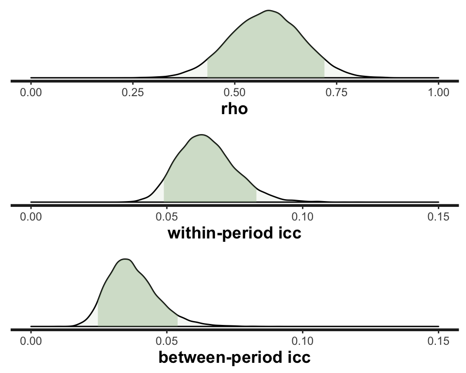

Decaying between-period ICC over time

Now we enter somewhat uncharted territory, since there is no obvious way in R using the lme4 or nlme packages to decompose the variance estimates when the random effects have correlation that decays over time. This is where we might have to rely on a Bayesian approach to do this. (I understand that SAS can accommodate this, but I can’t bring myself to go there.)

We start where we pretty much always do - generating the data. Everything is the same, except that the cluster-random effects are correlated over time; we specify a correlation structure of ar1 (auto-regressive).

set.seed(4119)
dar1 <- genDD(defc, defa, 60, 7, 4, 1, 2, 0.6, "ar1")

# correlation of "unobserved" random effects

round(cor(dcast(dar1[, .SD[1], keyby = .(cluster, period)], 
  formula = cluster ~ period, value.var = "cteffect")[, 2:7]), 2)

##      0    1    2    3    4    5
## 0 1.00 0.60 0.22 0.20 0.18 0.06
## 1 0.60 1.00 0.64 0.45 0.30 0.23
## 2 0.22 0.64 1.00 0.61 0.32 0.30
## 3 0.20 0.45 0.61 1.00 0.61 0.49
## 4 0.18 0.30 0.32 0.61 1.00 0.69
## 5 0.06 0.23 0.30 0.49 0.69 1.00

The model file is similar to nested_cor_cs.stan, except that the specifications of the variance-covariance matrix and ICC’s are now a function of \(\rho^{|t^\prime - t|}\):

transformed parameters{ 
  ⋮
  for (j in 1:T)
    for (k in 1:T)
      Sigma[j,k] = pow(sigmalev1,2) * pow(rho,abs(j-k));
  ⋮
}

generated quantities {
  ⋮
  for (j in 1:T)
      for (k in 1:T)
        icc[j, k] = sigmalev12/(sigmalev12 + sigma2) * pow(rho,abs(j-k));
  ⋮
}

The stan compilation and sampling code is not shown here - they are the same before. The posterior distribution of \(\rho\) is similar to what we saw previously.

print(fit.ar1, pars=c("rho"))

## Inference for Stan model: nested_cor_ar1.
## 4 chains, each with iter=5000; warmup=1000; thin=1; 
## post-warmup draws per chain=4000, total post-warmup draws=16000.
## 
##     mean se_mean   sd 2.5%  25%  50%  75% 97.5% n_eff Rhat
## rho 0.58       0 0.08 0.41 0.53 0.58 0.64  0.73  2302    1
## 
## Samples were drawn using NUTS(diag_e) at Fri Jun 28 14:13:41 2019.
## For each parameter, n_eff is a crude measure of effective sample size,
## and Rhat is the potential scale reduction factor on split chains (at 
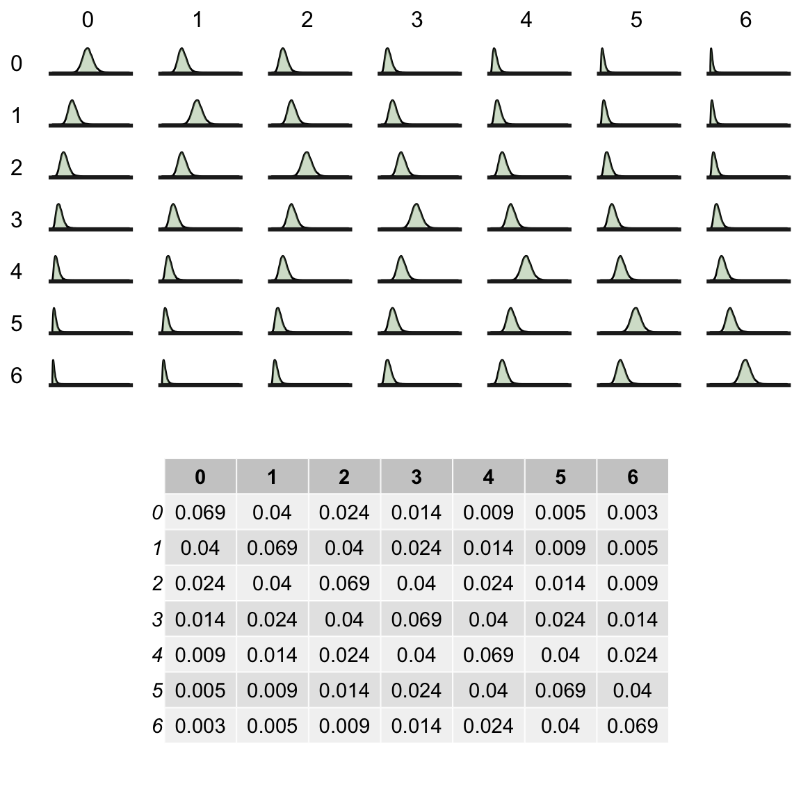
## convergence, Rhat=1).

Now, however, we have to consider a full range of ICC estimates. Here is a plot of the posterior distribution of all ICC’s with the means of each posterior directly below. The diagonal represents the within-period (constant) ICCs, and the off-diagonals are the between-period ICC’s.

An alternative Bayesian model: unstructured correlation

Now, there is no particular reason to expect that the particular decay model (with an AR1 structure) would be the best model. We could try to fit an even more general model, one with minimal structure. For example if we put no restrictions on the correlation matrix \(\mathbf{R}\), but assumed a constant variance of \(\sigma_b^2\), we might achieve a better model fit. (We could go even further and relax the assumption that the variance across time changes as well, but I’ll leave that to you if you want to try it.)

In this case, we need to define \(\mathbf{R}\) and specify a prior distribution (I use the Lewandowski, Kurowicka, and Joe - LKJ prior, as suggested by Stan documentation) and define the ICC’s in terms of \(\mathbf{R}\). Here are the relevant snippets of the stan model (everything else is the same as before):

parameters {
  ⋮
  corr_matrix[T] R;        // correlation matrix
  ⋮
}
 
transformed parameters{ 
  ⋮
  Sigma = pow(sigmalev1,2) * R;
  ⋮
}

model {
  ⋮
  R ~ lkj_corr(1);         // LKJ prior on the correlation matrix 
  ⋮
}

generated quantities {
  ⋮
  for (j in 1:T)
    for (k in 1:T)
      icc[j, k] = sigmalev12/(sigmalev12 + sigma2) * R[j, k];
  ⋮
}

Here are the means of the ICC posterior distributions alongside the means from the previous auto-regressive model.

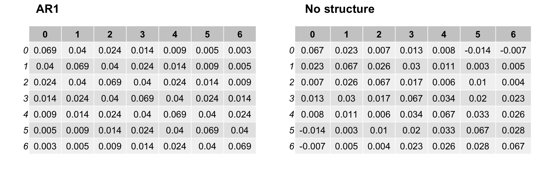
Looking at the unstructured model estimates on the right, it does appear that a decay model might be reasonable. (No surprise there, because in reality, it is totally reasonable; that’s how we generated the data.) We can use package bridgesampling which estimates marginal log likelihoods (across the prior distributions of the parameters). The marginal likelihoods are used in calculating the Bayes Factor, which is the basis for comparing two competing models. Here, the log-likelihood is reported. If the unstructured model is indeed an improvement (and it could very well be, because it has more parameters), the we would expect the marginal log-likelihood for the second model to be greater (less negative) than the log-likelihood for the auto-regressive model. If fact, the opposite true, suggesting the auto-regressive model is the preferred one (out of these two):

library(bridgesampling)

bridge_sampler(fit.ar1, silent = TRUE)

## Bridge sampling estimate of the log marginal likelihood: -5132.277
## Estimate obtained in 6 iteration(s) via method "normal"

bridge_sampler(fit.ar1.nc, silent = TRUE)

## Bridge sampling estimate of the log marginal likelihood: -5137.081
## Estimate obtained in 269 iteration(s) via method "normal".

Addendum - interpreting lmer variance estimates

In order to show how the lmer variance estimates relate to the theoretical variances and correlations in the case of a constant between-period ICC, here is a simulation based on 1000 clusters. The key parameters are \(\sigma^2_b = 0.15\), \(\sigma^2_e = 2\), and \(\rho = 0.6\). And based on these values, the theoretical ICC’s are: \(ICC_{within} = 0.15/2.15 = 0.698\), and \(ICC_{bewteen} = 0.698 * 0.6 = 0.042\).

set.seed(4119)
dcs <- genDD(defc, defa, 1000, 7, 4, 1, 2, 0.6, "cs")

The underlying correlation matrix of the cluster-level effects is what we would expect:

round(cor(dcast(dcs[, .SD[1], keyby = .(cluster, period)], 
  formula = cluster ~ period, value.var = "cteffect")[, 2:7]), 2)

##      0    1    2    3    4    5
## 0 1.00 0.59 0.59 0.61 0.61 0.61
## 1 0.59 1.00 0.61 0.60 0.61 0.64
## 2 0.59 0.61 1.00 0.59 0.61 0.61
## 3 0.61 0.60 0.59 1.00 0.59 0.62
## 4 0.61 0.61 0.61 0.59 1.00 0.60
## 5 0.61 0.64 0.61 0.62 0.60 1.00

Here are the variance estimates from the mixed-effects model:

lmerfit <- lmer(Y ~ period + rx + (1 | cluster/period) , data = dcs)
as.data.table(VarCorr(lmerfit))

##               grp        var1 var2       vcov     sdcor
## 1: period:cluster (Intercept) <NA> 0.05779349 0.2404028
## 2:        cluster (Intercept) <NA> 0.09143749 0.3023863
## 3:       Residual        <NA> <NA> 1.98894356 1.4102991

The way lmer implements the nested random effects , the cluster period-specific effect \(b_{ct}\) is decomposed into \(v_c\), a cluster level effect, and \(w_{ct}\), a cluster time-specific effect:

\[ b_{ct} = v_c + w_{ct} \]

Since both \(v_c\) and \(w_{ct}\) are normally distributed (\(v_c \sim N(0,\sigma_v^2)\) and \(w_{ct} \sim N(0,\sigma_w^2)\)), \(var(b_{ct}) = \sigma^2_b = \sigma^2_v + \sigma^2_w\).

Here is the observed estimate of \(\sigma^2_v + \sigma^2_w\):

vs <- as.data.table(VarCorr(lmerfit))$vcov
sum(vs[1:2])

## [1] 0.149231

An estimate of \(\rho\) can be extracted from the lmer model variance estimates:

\[ \begin{aligned} \rho &= cov(b_{ct}, b_{ct^\prime}) \\ &= cov(v_{c} + w_{ct}, v_{c} + w_{ct^\prime}) \\ &= var(v_c) + cov(w_{ct}) \\ &= \sigma^2_v \end{aligned} \]

\[ \begin{aligned} var(b_{ct}) &= var(v_{c}) + var(w_{ct}) \\ &= \sigma^2_v + \sigma^2_w \end{aligned} \]

\[ \begin{aligned} cor(b_{ct}, b_{ct^\prime}) &= \frac{cov(b_{ct}, b_{ct^\prime})}{\sqrt{var(b_{ct}) var(b_{ct^\prime})} } \\ \rho &= \frac{\sigma^2_v}{\sigma^2_v + \sigma^2_w} \end{aligned} \]

vs[2]/sum(vs[1:2])

## [1] 0.6127246

And here are the estimates of within and between-period ICC’s:

\[ICC_{tt} = \frac{\sigma^2_b}{\sigma^2_b+\sigma^2_e} =\frac{\sigma^2_v + \sigma^2_w}{\sigma^2_v + \sigma^2_w+\sigma^2_e}\]

sum(vs[1:2])/sum(vs)

## [1] 0.06979364

\[ \begin{aligned} ICC_{tt^\prime} &= \left( \frac{\sigma^2_b}{\sigma^2_b+\sigma^2_e}\right) \rho \\ \\ &= \left( \frac{\sigma^2_v + \sigma^2_w}{\sigma^2_v + \sigma^2_w+\sigma^2_e}\right) \rho \\ \\ &=\left( \frac{\sigma^2_v + \sigma^2_w}{\sigma^2_v + \sigma^2_w+\sigma^2_e} \right) \left( \frac{\sigma^2_v}{\sigma^2_v + \sigma^2_w} \right) \\ \\ &= \frac{\sigma^2_v}{\sigma^2_v + \sigma^2_w+\sigma^2_e} \end{aligned} \]

vs[2]/sum(vs)

## [1] 0.04276428