I am always saying that simulation can help illuminate interesting statistical concepts or ideas. Such an exploration might provide some insight into the concept of the design effect, which underlies clustered randomized trial designs. I’ve written about clustered-related methods so much on this blog that I won’t provide links - just peruse the list of entries on the home page and you are sure to spot a few. But, I haven’t written explicitly about the design effect.
When individual outcomes in a group are correlated, we learn less about the group from adding a new individual than we might think. Take an extreme example where every individual in a group is perfectly correlated with all the others: we will learn nothing new about the group by adding someone new. In fact, we might as well just look at a single member, since she is identical to all the others. The design effect is a value that in a sense quantifies how much information we lose (or, surprisingly, possibly gain) by this interdependence.
Let’s just jump right into it.
The context
Imagine a scenario where an underlying population of interest is structurally defined by a group of clusters. The classic case is students in schools or classrooms. I don’t really do any school-based education (I learned from debating my teacher-wife that is a dangerous area to tread), but this example seems so clear. (The ideas in this post were, in part, motivated by my involvement with the NIA IMPACT Collaboratory, which focuses at the opposite end of life, seeking to improve care and quality of life for people living with advanced dementia and their caregivers through research and pragmatic clinical trials.) We might be interested in measuring the effect of some intervention (it may or may not take place in school) on an educational attainment outcome of high school-aged kids in a city (I am assuming a continuous outcome here just because it is so much easier to visualize). It does not seem crazy to think that the outcomes of kids from the same school might be correlated, either because the school itself does such a good (or poor) job of teaching or similar types of kids tend to go to the same school.
The unit of randomization
We have at least three ways to design our study. We could just recruit kids out and about in city and randomize them each individually to intervention or control. In the second approach, we decide that it is easier to randomize the schools to intervention or control - and recruit kids from each of the schools. This means that all kids from one school will be in the same intervention arm. And for the third option, we can go half way: we go to each school and recruit kids, randomizing half of the kids in each school to control, and the other half to the intervention. This last option assumes that we could ensure that the kids in the school exposed to the intervention would not influence their unexposed friends.
In all three cases the underlying assumptions are the same - there is a school effect on the outcome, an individual effect, and an intervention effect. But it turns out that the variability of the intervention effect depends entirely on how we randomize. And since variability of the outcome affects sample size, each approach has implications for sample size. (I’ll point you to a book by Donner & Klar, which gives a comprehensive and comprehensible overview of cluster randomized trials.)
Simulation of each design
Just to be clear about these different randomization designs, I’ll simulate 1500 students using each. I’ve set a seed in case you’d like to recreate the results shown here (and indicate the libraries I am using).
library(simstudy)
library(data.table)
library(ggplot2)
library(clusterPower)
library(parallel)
library(lmerTest)

RNGkind("L'Ecuyer-CMRG") # enables seed for parallel process
set.seed(987)
Randomization by student
I’ve written a function for each of the three designs to generate the data, because later I am going to need to generate multiple iterations of each design. In the first case, randomization is applied to the full group of students:
independentData <- function(N, d1) {

  di <- genData(N)
  di <- trtAssign(di, grpName = "rx")
  di <- addColumns(d1, di)
  di[]

}
The outcome is a function of intervention status and a combined effect of the student’s school and the student herself. We cannot disentangle the variance components, because we do not know the identity of the school:
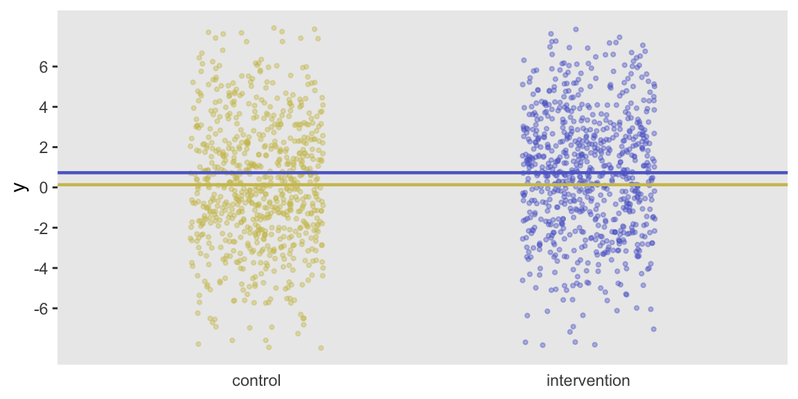
defI1 <- defDataAdd(varname = "y", formula = "0.8 * rx",
                variance = 10, dist = "normal")

dx <- independentData(N = 30 * 50, defI1)
The observed effect size and variance should be close to the specified parameters of 0.8 and 10, respectively:
dx[rx == 1, mean(y)] - dx[rx == 0, mean(y)]## [1] 0.597dx[, var(y)]## [1] 10.2Here is a plot of the individual observations that highlights the group differences and individual variation:
Randomization by site
Next, the intervention status is assigned to each of the \(k\) schools/clusters before generating \(m\) students per cluster. In this case, the outcome (defined by defI2) is a function of the cluster effect, individual effect, and the intervention status. Note here, the variance components are disentangled, but together they sum to 10, suggesting that total variance should be the same as the first scenario:
clusteredData <- function(k, m, d1, d2) {

  dc <- genData(k, d1)
  dc <- trtAssign(dc, grpName = "rx")

  di <- genCluster(dc, "site", m, level1ID = "id")
  di <- addColumns(d2, di)
  di[]

}
defC <- defData(varname = "ceff", formula = 0,
variance = 0.5, id = "site", dist = "normal")
defI2 <- defDataAdd(varname = "y", formula = "ceff + 0.8 * rx",
variance = 9.5, dist = "normal")dx <- clusteredData(k = 30, m = 50, defC, defI2)The effect size and variation across all observations should be be quite similar to the previous design, though now the data has a structure that is determined by the clusters:
dx[rx == 1, mean(y)] - dx[rx == 0, mean(y)]## [1] 0.203dx[, var(y)]## [1] 10.5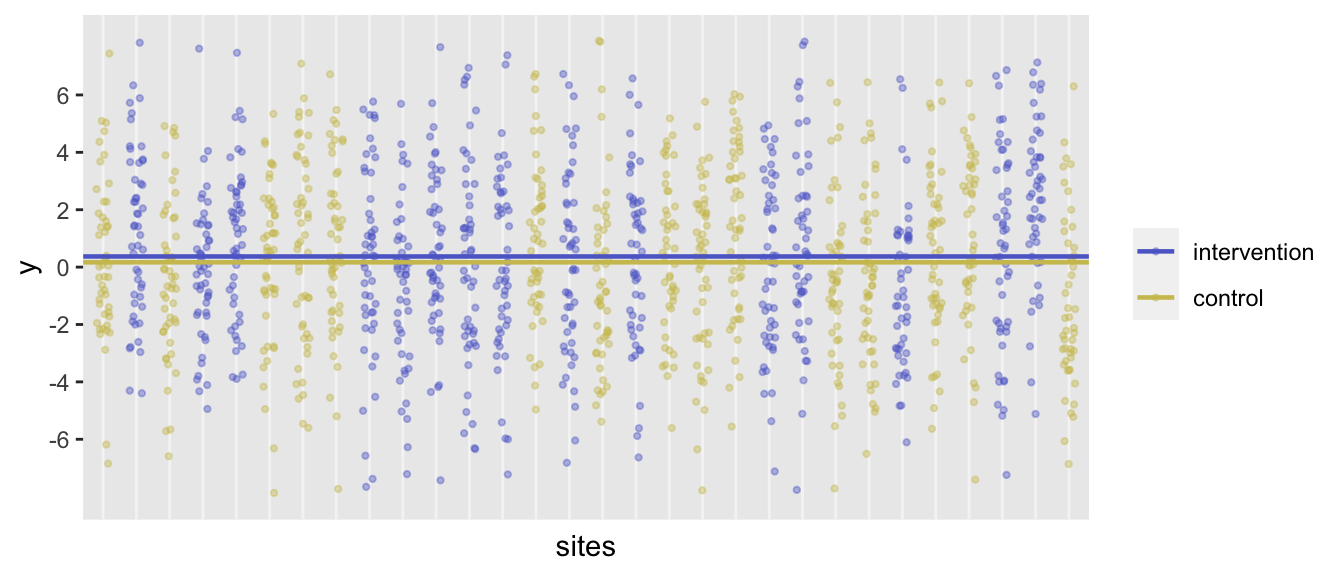
Randomization within site
In the last design, the treatment assignment is made after both the clusters and individuals have been generated. Cluster randomization within site is specified using the strata argument:
withinData <- function(k, m, d1, d2) {

  dc <- genData(k, d1)

  di <- genCluster(dc, "site", m, "id")
  di <- trtAssign(di, strata="site", grpName = "rx")
  di <- addColumns(d2, di)

  di[]

}
dx <- withinData(30, 50, defC, defI2)
dx[rx == 1, mean(y)] - dx[rx == 0, mean(y)]## [1] 0.813dx[, var(y)]## [1] 10.1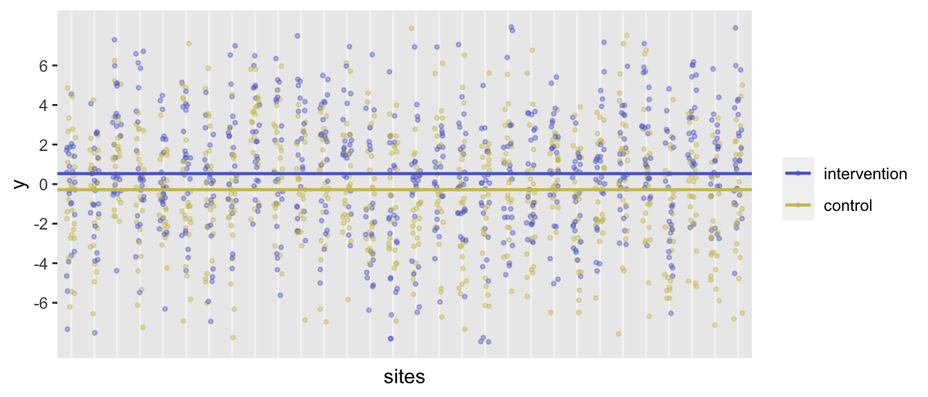
The design effect
There’s a really nice paper by Vierron & Giraudeau that describes many of the issues I am only touching on here. In particular, they define the design effect and then relate this definition to formulas that are frequently used simplify the estimation of the design effect.
Consider the statistics \(\sigma^2_{\Delta_{bc}}\) and \(\sigma^2_{\Delta_{i}}\), which are the variance of the effect sizes under the cluster randomization and the individual randomization designs, respectively:
\[\sigma^2_{\Delta_{bc}} = Var(\bar{Y}_1^{bc} - \bar{Y}_0^{bc})\]
and
\[\sigma^2_{\Delta_{i}} =Var(\bar{Y}_1^{i} - \bar{Y}_0^{i})\]
These variances are never observed, since they are based on a very large (really, an infinite) number of repeated experiments. However, the theoretical variances can be derived (as they are in the paper), and can be simulated (as they will be here). The design effect \(\delta_{bc}\) is defined as
\[\delta_{bc} = \frac{\sigma^2_{\Delta_{bc}}}{\sigma^2_{\Delta_{i}}}\]
This ratio represents the required adjustment in sample size required to make the two designs equivalent in the sense that they provide the same amount of information. This will hopefully become clear with the simulations below.
I have decided to use \(k = 50\) clusters to ensure a large enough sample size to estimate the proper variance. I need to know how many individuals per cluster are required for 80% power in the cluster randomized design, given the effect size and variance assumptions I’ve been using here. I’ll use the clusterPower package (which unfortunately defines the number of clusters in each as \(m\), so don’t let that confuse you). Based on this, we should have 18 students per school, for a total sample of 900 students:
crtpwr.2mean(m = 50/2, d = 0.8, icc = 0.05, varw = 9.5)## n
## 17.9Now, I am ready to generate effect sizes for each of 2000 iterations of the experiment assuming randomization by cluster. With this collection of effect sizes in hand, I will be able to estimate their variance:
genDifFromClust <- function(k, m, d1, d2) {
  dx <- clusteredData(k, m, d1, d2)
  dx[rx == 1, mean(y)] - dx[rx == 0, mean(y)]
}

resC <- unlist(mclapply(1:niters,
   function(x) genDifFromClust(k= 50, m=18, defC, defI2)))
Here is an estimate of \(\sigma^2_{\Delta_{bc}}\) based on the repeated experiments:
(s2.D_bc <- var(resC))## [1] 0.0818And here is the estimate of \(\sigma^2_{\Delta_{i}}\) (the variance of the effect sizes based on individual-level randomization experiments):
genDifFromInd <- function(N, d1) {
  dx <- independentData(N, d1)
  dx[rx == 1, mean(y)] - dx[rx == 0, mean(y)]
}

resI <- unlist(mclapply(1:niters,
          function(x) genDifFromInd(N = 50*18, defI1)))

(s2.D_i <- var(resI))
## [1] 0.0432So, now we can use these variance estimates to derive the estimate of the design effect \(\delta_{bc}\), which, based on the earlier definition, is:
(d_bc <- s2.D_bc / s2.D_i)## [1] 1.89The Vierron & Giraudeau paper derives a simple formula for the design effect assuming equal cluster sizes and an ICC \(\rho\). This (or some close variation, when cluster sizes are not equal) is quite commonly used:
\[\delta_{bc} = 1 + (m-1)*\rho\]
As the ICC increases, the design effect increases. Based on the parameters for \(m\) and \(\rho\) we have been using in these simulations (note that \(\rho = 0.5/(0.5+9.5) = 0.05\)), the standard formula gives us this estimate of \(\delta_{bc.formula}\) that is quite close to our experimental value:
( d_bc_form <- 1 + (18-1) * (0.05) )## [1] 1.85
But what is the design effect?
OK, finally, we can now see what the design effect actually represents. As before, we will generate repeated data sets; this time, we will estimate the treatment effect using an appropriate model. (In the case of the cluster randomization, this is a linear mixed effects model, and in the case of individual randomization, this is linear regression model.) For each iteration, I am saving the p-value for the treatment effect parameter in the model. We expect close to 80% of the p-values to be lower than 0.05 (this is 80% power given a true treatment effect of 0.8).
First, here is the cluster randomized experiment and the estimate of power:
genEstFromClust <- function(k, m, d1, d2) {
  dx <- clusteredData(k, m, d1, d2)
  summary(lmerTest::lmer(y ~ rx + (1|site), data = dx))$coef["rx", 5]
}

resCest <- unlist(mclapply(1:niters,
          function(x) genEstFromClust(k=50, m = 18, defC, defI2)))

mean(resCest < 0.05) # power
## [1] 0.778In just over 80% of the cases, we would have rejected the null.
And here is the estimated power under the individual randomization experiment, but with a twist. Since the design effect is 1.85, the cluster randomized experiment needs a relative sample size 1.85 times higher than an equivalent (individual-level) RCT to provide the same information, or to have equivalent power. So, in our simulations, we will use a reduced sample size for the individual RCT. Since we used 900 individuals in the CRT, we need only \(900/1.85 = 487\) individuals in the RCT:
( N.adj <- ceiling( 50 * 18 / d_bc_form ) )## [1] 487genEstFromInd <- function(N, d1) {
dx <- independentData(N, d1)
summary(lm(y ~ rx, data = dx))$coef["rx", 4]
}
resIest <- unlist(mclapply(1:niters,
function(x) genEstFromInd(N = N.adj, defI1)))The power for this second experiment is also quite close to 80%:
mean(resIest < 0.05) # power## [1] 0.794Within cluster randomization
It is interesting to see what happens when we randomize within the cluster. I think there may be some confusion here, because I have seen folks incorrectly apply the standard formula for \(\delta_{bc}\), rather than this formula for \(\delta_{wc}\) that is derived (again, under the assumption of equal cluster sizes) in the Vierron & Giraudeau paper as
\[ \delta_{wc} = 1- \rho\]
This implies that the sample size requirement actually declines as intra-cluster correlation increases! In this case, since \(\rho = 0.05\), the total sample size for the within-cluster randomization needs to be only 95% of the sample size for the individual RCT.
As before, let’s see if the simulated data confirms this design effect based on the definition
\[ \delta_{wc} = \frac{\sigma^2_{\Delta_{wc}}}{\sigma^2_{\Delta_{i}}}\]
genDifFromWithin <- function(k, m, d1, d2) {
  dx <- withinData(k, m, d1, d2)
  dx[rx == 1, mean(y)] - dx[rx == 0, mean(y)]
}

resW <- unlist(mclapply(1:niters,
   function(x) genDifFromWithin(k = 50, m = 18, defC, defI2)))

(s2.D_wc <- var(resW))
## [1] 0.0409The estimated design effect is quite close to the expected design effect of 0.95:
(d_wc <- s2.D_wc / s2.D_i)## [1] 0.947And to finish things off, if we estimate an adjusted cluster size based on the design effects (first reducing the cluster size \(m=18\) for the cluster randomized trial by \(\delta_{bc.formula}\) to derive the appropriate sample size for the RCT, and then adjusting by \(\delta_{wc} = 0.95\)) to get the appropriate cluster size for the within cluster randomization, which is about 9 students. This study will only have 450 students, fewer than the RCT:
(m.adj <- round( (18 / d_bc_form) * 0.95, 0))## [1] 9genEstFromWithin <- function(k, m, d1, d2) {
dx <- withinData(k, m, d1, d2)
summary(lmerTest::lmer(y ~ rx + (1|site), data = dx))$coef["rx", 5]
}
resWest <- unlist(mclapply(1:niters,
function(x) genEstFromWithin(k = 50, m = ceiling(m.adj), defC, defI2)))
mean(resWest < 0.05)## [1] 0.779
References:
Donner, Allan, and Neil Klar. “Design and analysis of cluster randomization trials in health research.” New York (2010).
Vierron, Emilie, and Bruno Giraudeau. “Design effect in multicenter studies: gain or loss of power?.” BMC medical research methodology 9, no. 1 (2009): 39.
Support:
This work was supported in part by the National Institute on Aging (NIA) of the National Institutes of Health under Award Number U54AG063546, which funds the NIA IMbedded Pragmatic Alzheimer’s Disease and AD-Related Dementias Clinical Trials Collaboratory (NIA IMPACT Collaboratory). The author, a member of the Design and Statistics Core, was the sole writer of this blog post and has no conflicts. The content is solely the responsibility of the author and does not necessarily represent the official views of the National Institutes of Health.