I frequently find myself in discussions with collaborators about the merits of reporting p-values, particularly in the context of pilot studies or exploratory analysis. Over the past several years, the American Statistical Association has made several strong statements about the need to consider approaches that measure the strength of evidence or uncertainty that don’t necessarily rely on p-values. In 2016, the ASA attempted to clarify the proper use and interpretation of the p-value by highlighting key principles “that could improve the conduct or interpretation of quantitative science, according to widespread consensus in the statistical community.” These principles are worth noting here in case you don’t make it over to the original paper:
- p-values can indicate how incompatible the data are with a specified statistical model.
- p-values do not measure the probability that the studied hypothesis is true, or the probability that the data were produced by random chance alone.
- scientific conclusions and business or policy decisions should not be based only on whether a p-value passes a specific threshold.
- proper inference requires full reporting and transparency
- a p-value, or statistical significance, does not measure the size of an effect or the importance of a result.
- by itself, a p-value does not provide a good measure of evidence regarding a model or hypothesis.
More recently, the ASA elaborated on this, responding to those who thought the initial paper was too negative, a list of many things not to do. In this new paper, the ASA argues that “knowing what not to do with p-values is indeed necessary, but it does not suffice.” We also need to know what we should do. One of those things should be focusing on effect sizes (and some measure of uncertainty, such as a confidence or credible interval) in order to evaluate an intervention or exposure.
Applying principled thinking to a small problem
Recently, I was discussing the presentation of results for a pilot study. I was arguing that we should convey the findings in a way that highlighted the general trends without leading readers to make overly strong conclusions, which p-values might do. So, I was arguing that, rather than presenting p-values, we should display effect sizes and confidence intervals, and avoid drawing on the concept of “statistical significance.”
Generally, this is not a problem; we can estimate an effect size like a difference in means, a difference in proportions, a ratio of proportions, a ratio of odds, or even the log of a ratio of odds. In this case, the outcome was a Likert-type survey where the response was “none”, “a little”, and “a lot”, and there were three comparison groups, so we had a \(3\times3\) contingency table with one ordinal (i.e. ordered) factor. In this case, it is not so clear what the effect size measurement should be.
One option is to calculate a \(\chi^2\) statistic, report the associated p-value, and call it a day. However, since the \(\chi^2\) is not a measure of effect and the p-value is not necessarily a good measure of evidence, I considered estimating a cumulative odds model that would provide a measure of the association between group and response. However, I was a little concerned, because the typical version of this model makes an assumption of proportional odds, which I wasn’t sure would be appropriate here. (I’ve written about these models before, here and here, if you want to take a look.) It is possible to fit a cumulative odds model without the proportionality assumption, but then the estimates are harder to interpret since the effect size varies by group and response.
Fortunately, there is a more general measure of association for contingency tables with at least one, but possibly two, nominal factors: Cramer’s V. This measure which makes no assumptions about proportionality.
My plan is to simulate contingency table data, and in this post, I will explore the cumulative odds models. Next time, I’ll describe the Cramer’s V measure of association.
Non-proportional cumulative odds
In the cumulative odds model (again, take a look here for a little more description of these models), we assume that all the log-odds ratios are proportional. This may actually not be an unreasonable assumption, but I wanted to start with a data set that is generated without explicitly assuming proportionality. In the following data definition, the distribution of survey responses (none, a little, and a lot) across the three groups (1, 2, and 3) are specified uniquely for each group:
library(simstudy)

# define the data

def <- defData(varname = "grp",
            formula = "0.3; 0.5; 0.2", dist = "categorical")

defc <- defCondition(condition = "fgrp == 1",
            formula = "0.70; 0.20; 0.10", dist = "categorical")
defc <- defCondition(defc, condition = "fgrp == 2",
            formula = "0.10; 0.60; 0.30", dist = "categorical")
defc <- defCondition(defc, condition = "fgrp == 3",
            formula = "0.05; 0.25; 0.70", dist = "categorical")

# generate the data

set.seed(99)

dx <- genData(180, def)
dx <- genFactor(dx, "grp", replace = TRUE)
dx <- addCondition(defc, dx, "rating")
dx <- genFactor(dx, "rating", replace = TRUE,
         labels = c("none", "a little", "a lot"))

dx[]
## id fgrp frating
## 1: 1 2 a little
## 2: 2 3 a little
## 3: 3 3 a lot
## 4: 4 2 a little
## 5: 5 2 a little
## ---
## 176: 176 2 a lot
## 177: 177 1 none
## 178: 178 3 a lot
## 179: 179 2 a little
## 180: 180 2 a littleA distribution plot based on these 180 observations indicates that the odds are not likely proportional; the “tell” is the large bulge for those in group 2 who respond a little.
library(likert)

items <- dx[, .(frating)]
names(items) <- c(frating = "rating")

likert.data <- likert(items = items, grouping = dx$fgrp)
plot(likert.data, wrap = 100, low.color = "#DAECED",
  high.color = "#CECD7B")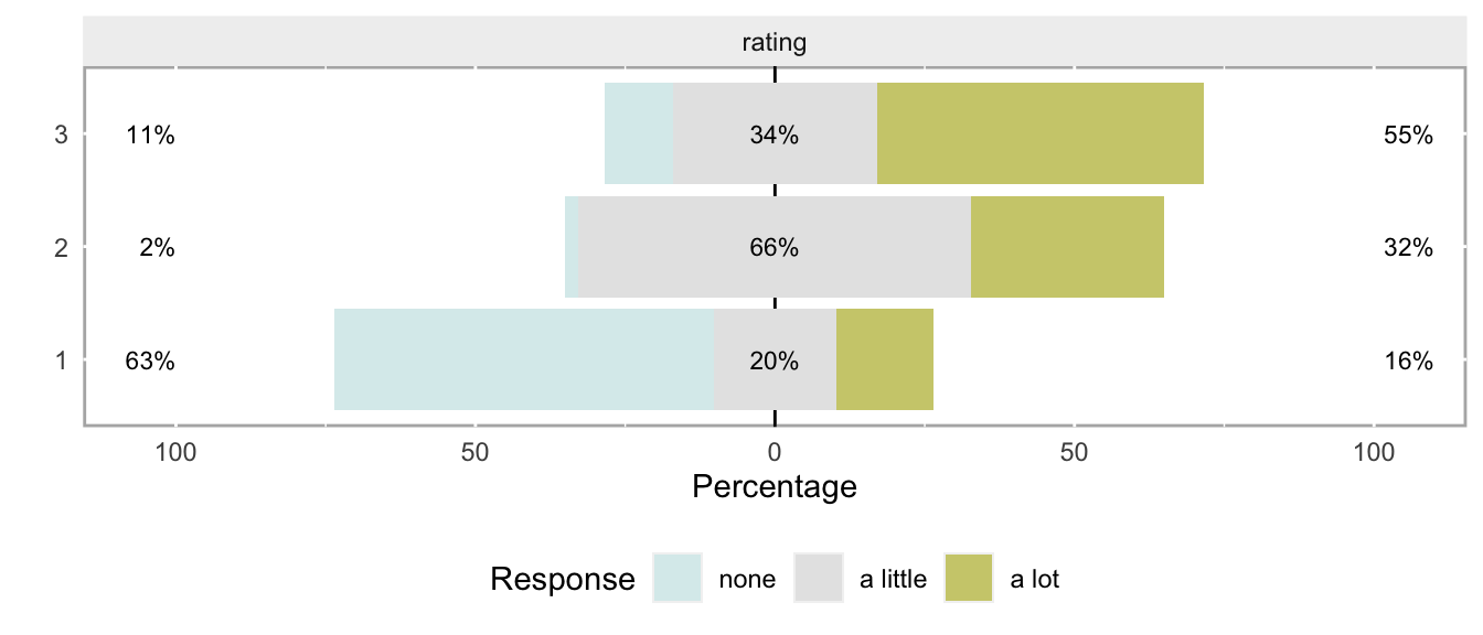
The \(\chi^2\) test, not so surprisingly, indicates that it would be reasonable to conclude there are differences in responses across the three groups:
chisq.test(table(dx[, .(fgrp, frating)]))##
## Pearson's Chi-squared test
##
## data: table(dx[, .(fgrp, frating)])
## X-squared = 84, df = 4, p-value <2e-16But, since we are trying to provide a richer picture of the association that will be less susceptible to small sample sizes, here is the cumulative (proportional) odds model fit using the clm function in the ordinal package.
library(ordinal)

clmFit.prop <- clm(frating ~ fgrp, data = dx)
summary(clmFit.prop)
## formula: frating ~ fgrp
## data: dx
##
## link threshold nobs logLik AIC niter max.grad cond.H
## logit flexible 180 -162.95 333.91 5(0) 4.61e-08 2.8e+01
##
## Coefficients:
## Estimate Std. Error z value Pr(>|z|)
## fgrp2 2.456 0.410 5.98 2.2e-09 ***
## fgrp3 3.024 0.483 6.26 3.9e-10 ***
## ---
## Signif. codes: 0 '***' 0.001 '**' 0.01 '*' 0.05 '.' 0.1 ' ' 1
##
## Threshold coefficients:
## Estimate Std. Error z value
## none|a little 0.335 0.305 1.10
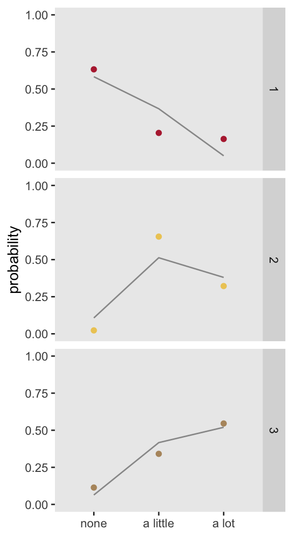
## a little|a lot 2.945 0.395 7.45A plot of the observed proportions (show by the line) with the modeled proportions (shown as points) indicates that the model that makes the proportional assumption might not be doing a great job:
If we fit a model that does not make the proportionality assumption and compare using either AIC statistic (lower is better) or a likelihood ratio test (small p-value indicates that the saturated/non-proportional model is better), it is clear that the non-proportional odds model for this dataset is a better fit.
clmFit.sat <- clm(frating ~ 1, nominal = ~ fgrp, data = dx)
summary(clmFit.sat)
## formula: frating ~ 1
## nominal: ~fgrp
## data: dx
##
## link threshold nobs logLik AIC niter max.grad cond.H
## logit flexible 180 -149.54 311.08 7(0) 8.84e-11 4.7e+01
##
## Threshold coefficients:
## Estimate Std. Error z value
## none|a little.(Intercept) 0.544 0.296 1.83
## a little|a lot.(Intercept) 1.634 0.387 4.23
## none|a little.fgrp2 -4.293 0.774 -5.54
## a little|a lot.fgrp2 -0.889 0.450 -1.98
## none|a little.fgrp3 -2.598 0.560 -4.64
## a little|a lot.fgrp3 -1.816 0.491 -3.70anova(clmFit.prop, clmFit.sat)## Likelihood ratio tests of cumulative link models:
##
## formula: nominal: link: threshold:
## clmFit.prop frating ~ fgrp ~1 logit flexible
## clmFit.sat frating ~ 1 ~fgrp logit flexible
##
## no.par AIC logLik LR.stat df Pr(>Chisq)
## clmFit.prop 4 334 -163
## clmFit.sat 6 311 -150 26.8 2 1.5e-06 ***
## ---
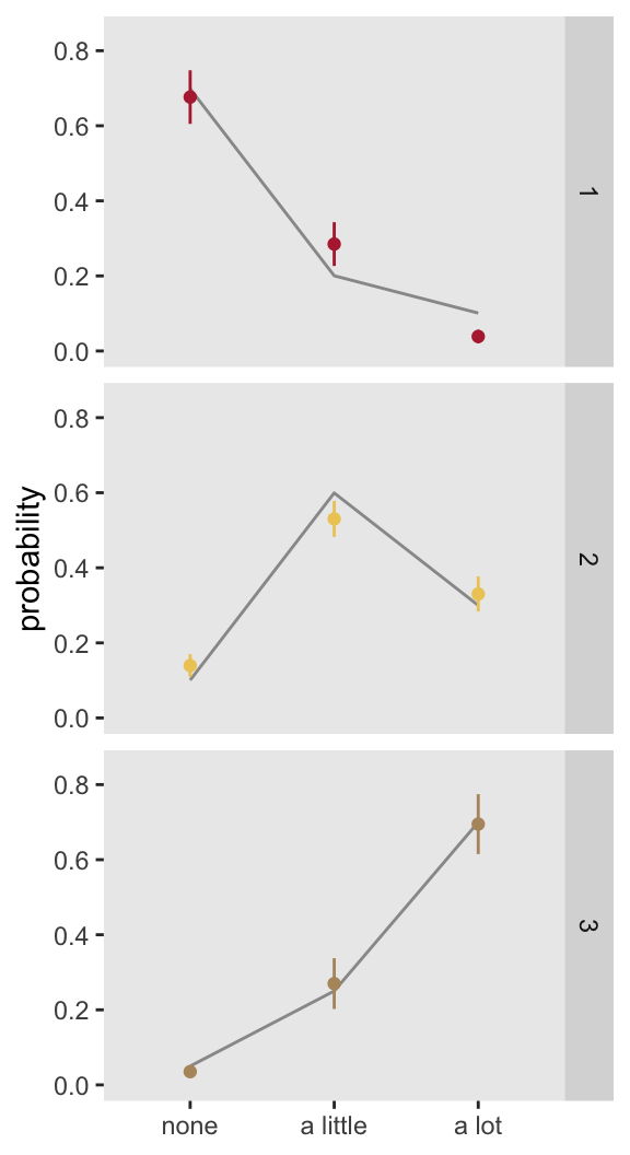
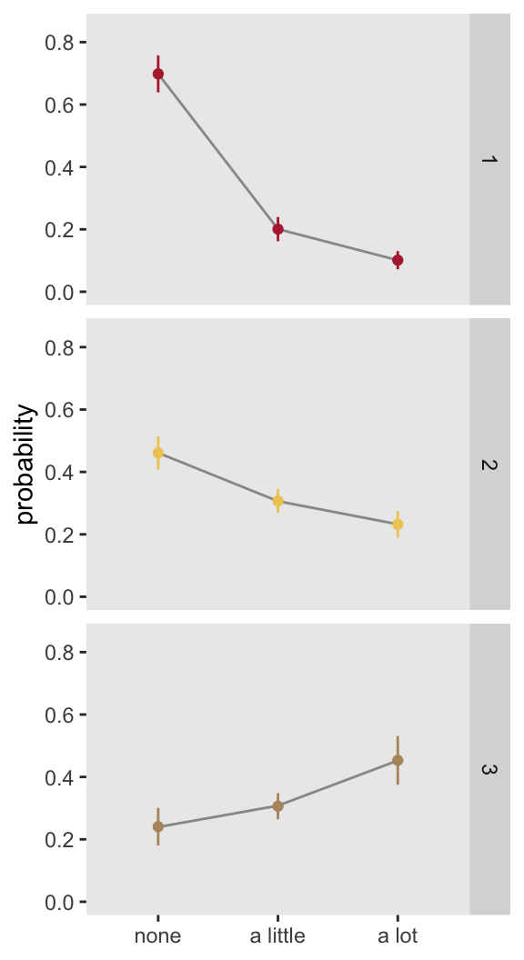
## Signif. codes: 0 '***' 0.001 '**' 0.01 '*' 0.05 '.' 0.1 ' ' 1It is possible that the poor fit is just a rare occurrence. Below is a plot that shows the average result (\(\pm 1 \ sd\)) for 1000 model fits for 1000 data sets using the same data generation process. It appears those initial results were not an aberration - the proportional odds model fits a biased estimate, particularly for groups 1 and 2. (The code to do this simulation is shown in the addendum.)
Proportional assumption fulfilled
Here the data generation process is modified so that the proportionality assumption is incorporated.
def <- defData(varname = "grp", formula = ".3;.5;.2",
dist = "categorical")
def <- defData(def, varname = "z", formula = "1*I(grp==2) + 2*I(grp==3)",
dist = "nonrandom")
baseprobs <- c(0.7, 0.2, 0.1)
dx <- genData(180, def)
dx <- genFactor(dx, "grp", replace = TRUE)
dx <- genOrdCat(dx, adjVar = "z", baseprobs, catVar = "rating")
dx <- genFactor(dx, "rating", replace = TRUE,
labels = c("none", "a little", "a lot")
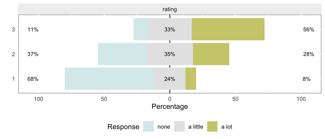
)This is what proportional odds looks like - there are no obvious bulges, just a general shift rightward as we move from group 1 to 3:
When we fit the proportional model and compare it to the saturated model, we see no reason to reject the assumption of proportionality (based on either the AIC or LR statistics).
clmFit.prop <- clm(frating ~ fgrp, data = dx)
summary(clmFit.prop)
## formula: frating ~ fgrp
## data: dx
##
## link threshold nobs logLik AIC niter max.grad cond.H
## logit flexible 180 -176.89 361.77 4(0) 3.04e-09 2.7e+01
##
## Coefficients:
## Estimate Std. Error z value Pr(>|z|)
## fgrp2 1.329 0.359 3.70 0.00022 ***
## fgrp3 2.619 0.457 5.73 1e-08 ***
## ---
## Signif. codes: 0 '***' 0.001 '**' 0.01 '*' 0.05 '.' 0.1 ' ' 1
##
## Threshold coefficients:
## Estimate Std. Error z value
## none|a little 0.766 0.299 2.56
## a little|a lot 2.346 0.342 6.86clmFit.sat <- clm(frating ~ 1, nominal = ~ fgrp, data = dx)
anova(clmFit.prop, clmFit.sat)## Likelihood ratio tests of cumulative link models:
##
## formula: nominal: link: threshold:
## clmFit.prop frating ~ fgrp ~1 logit flexible
## clmFit.sat frating ~ 1 ~fgrp logit flexible
##
## no.par AIC logLik LR.stat df Pr(>Chisq)
## clmFit.prop 4 362 -177
## clmFit.sat 6 365 -177 0.56 2 0.75And here is a plot summarizing a second set of 1000 iterations, this one using the proportional odds assumption. The estimates appear to be unbiased:
I suspect that in many instances, Likert-type responses will look more like the second case than the first case, so that the cumulative proportional odds model could very well be useful in characterizing the association between group and response. Even if the assumption is not reasonable, the bias might not be terrible, and the estimate might still be useful as a measure of association. However, we might prefer a measure that is free of any assumptions, such as Cramer’s V. I’ll talk about that next time.
References:
Ronald L. Wasserstein & Nicole A. Lazar (2016) The ASA Statement on p-Values: Context, Process, and Purpose, The American Statistician, 70:2, 129-133.
Ronald L. Wasserstein, Allen L. Schirm & Nicole A. Lazar (2019) Moving to a World Beyond “p < 0.05”, The American Statistician, 73:sup1, 1-19.
Addendum: code for replicated analysis
library(parallel)
RNGkind("L'Ecuyer-CMRG")  # to set seed for parallel process

dat.nonprop <- function(iter, n) {

  dx <- genData(n, def)
  dx <- genFactor(dx, "grp", replace = TRUE)
  dx <- addCondition(defc, dx, "rating")
  dx <- genFactor(dx, "rating", replace = TRUE,
            labels = c("none", "a little", "a lot")
  )

  clmFit <- clm(frating ~ fgrp, data = dx)

  dprob.obs <- data.table(iter,
      prop.table(dx[, table(fgrp, frating)], margin = 1))

  setkey(dprob.obs, fgrp, frating)
  setnames(dprob.obs, "N", "p.obs")

  dprob.mod <- data.table(iter, fgrp = levels(dx$fgrp),
      predict(clmFit, newdata = data.frame(fgrp = levels(dx$fgrp)))$fit)

  dprob.mod <- melt(dprob.mod, id.vars = c("iter", "fgrp"),
                    variable.name = "frating", value.name = "N")

  setkey(dprob.mod, fgrp, frating)
  setnames(dprob.mod, "N", "p.fit")

  dprob <- dprob.mod[dprob.obs]
  dprob[, frating := factor(frating,
                        levels=c("none", "a little", "a lot"))]

  dprob[]

}

def <- defData(varname = "grp", formula = ".3;.5;.2",
            dist = "categorical")

defc <- defCondition(condition = "fgrp == 1",
            formula = "0.7;0.2;0.1", dist = "categorical")
defc <- defCondition(defc, condition = "fgrp == 2",
            formula = "0.1;0.6;0.3", dist = "categorical")
defc <- defCondition(defc, condition = "fgrp == 3",
            formula = "0.05;0.25;0.70", dist = "categorical")

res.nonp <- rbindlist(mclapply(1:1000,
                        function(iter) dat.nonprop(iter,180)))

sum.nonp <- res.nonp[, .(mfit = mean(p.fit), sfit = sd(p.fit),
              mobs = mean(p.obs), sobs = sd(p.obs)),
              keyby = .(fgrp, frating)]

sum.nonp[, `:=`(lsd = mfit - sfit, usd = mfit + sfit)]

ggplot(data = sum.nonp, aes(x = frating, y = mobs)) +
  geom_line(aes(group = fgrp), color = "grey60") +
  geom_errorbar(aes(ymin = lsd, ymax = usd,  color = fgrp),
                width = 0) +
  geom_point(aes(y = mfit, color = fgrp)) +
  theme(panel.grid = element_blank(),
        legend.position = "none",
        axis.title.x = element_blank()) +
  facet_grid(fgrp ~ .) +
  scale_y_continuous(limits = c(0, 0.85), name = "probability") +
  scale_color_manual(values = c("#B62A3D", "#EDCB64", "#B5966D"))