In my last post, I made the point that p-values should not necessarily be considered sufficient evidence (or evidence at all) in drawing conclusions about associations we are interested in exploring. When it comes to contingency tables that represent the outcomes for two categorical variables, it isn’t so obvious what measure of association should augment (or replace) the \(\chi^2\) statistic.
I described a model-based measure of effect to quantify the strength of an association in the particular case where one of the categorical variables is ordinal. This can arise, for example, when we want to compare Likert-type responses across multiple groups. The measure of effect I focused on - the cumulative proportional odds - is quite useful, but is potentially limited for two reasons. First, the proportional odds assumption may not be reasonable, potentially leading to biased estimates. Second, both factors may be nominal (i.e. not ordinal), it which case cumulative odds model is inappropriate.
An alternative, non-parametric measure of association that can be broadly applied to any contingency table is Cramér’s V, which is calculated as
\[ V = \sqrt{\frac{\chi^2/N}{min(r-1, c-1)}} \] where \(\chi^2\) is from the Pearson’s chi-squared test, \(N\) is the total number of responses across all groups, \(r\) is the number of rows in the contingency table, and \(c\) is the number of columns. \(V\) ranges from \(0\) to \(1\), with \(0\) indicating no association, and \(1\) indicating the strongest possible association. (In the addendum, I provide a little detail as to why \(V\) cannot exceed \(1\).)
Simulating independence
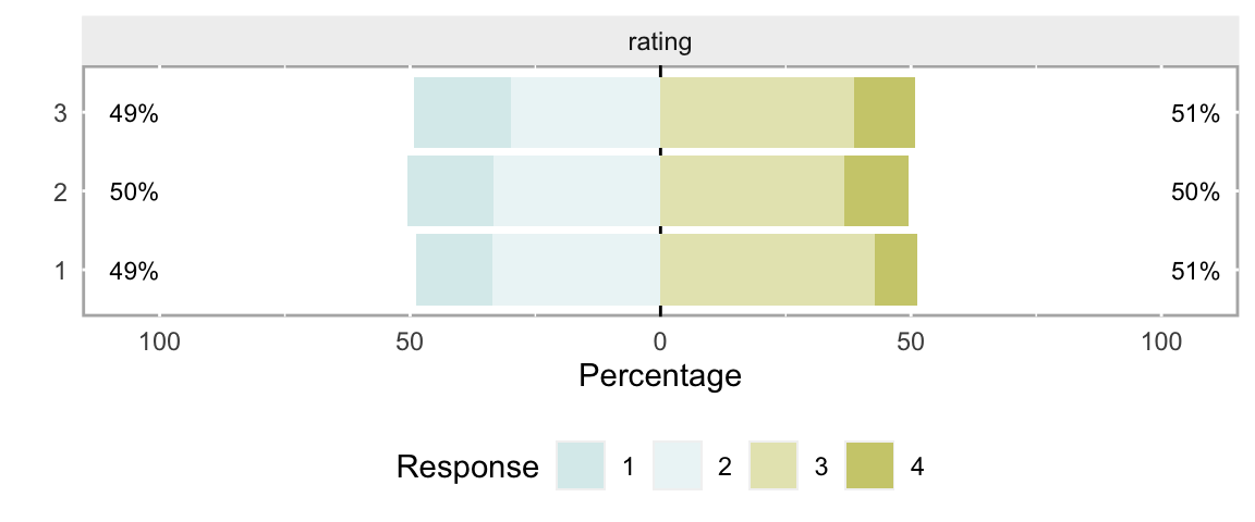
In this first example, the distribution of ratings is independent of the group membership. In the data generating process, the probability distribution for rating has no reference to grp, so we would expect similar distributions of the response across the groups:
library(simstudy)

def <- defData(varname = "grp",
         formula = "0.3; 0.5; 0.2", dist = "categorical")
def <- defData(def, varname = "rating",
         formula = "0.2;0.3;0.4;0.1", dist = "categorical")

set.seed(99)
dind <- genData(500, def)
And in fact, the distributions across the 4 rating options do appear pretty similar for each of the 3 groups:
In order to estimate \(V\) from this sample, we use the \(\chi^2\) formula (I explored the chi-squared test with simulations in a two-part post here and here):
\[ \sum_{i,j} {\frac{(O_{ij} - E_{ij})^2}{E_{ij}}} \]
observed <- dind[, table(grp, rating)]
obs.dim <- dim(observed)

getmargins <- addmargins(observed, margin = seq_along(obs.dim),
                         FUN = sum, quiet = TRUE)

rowsums <- getmargins[1:obs.dim[1], "sum"]
colsums <- getmargins["sum", 1:obs.dim[2]]

expected <- rowsums %*% t(colsums) / sum(observed)
X2 <- sum( ( (observed - expected)^2) / expected)

X2
## [1] 3.45And to check our calculation, here’s a comparison with the estimate from the chisq.test function:
chisq.test(observed)##
## Pearson's Chi-squared test
##
## data: observed
## X-squared = 3.5, df = 6, p-value = 0.8With \(\chi^2\) in hand, we can estimate \(V\), which we expect to be quite low:
sqrt( (X2/sum(observed)) / (min(obs.dim) - 1) )## [1] 0.05874Again, to verify the calculation, here is an alternative estimate using the DescTools package, with a 95% confidence interval:
library(DescTools)

CramerV(observed, conf.level = 0.95)
## Cramer V lwr.ci upr.ci
## 0.05874 0.00000 0.08426
Group membership matters
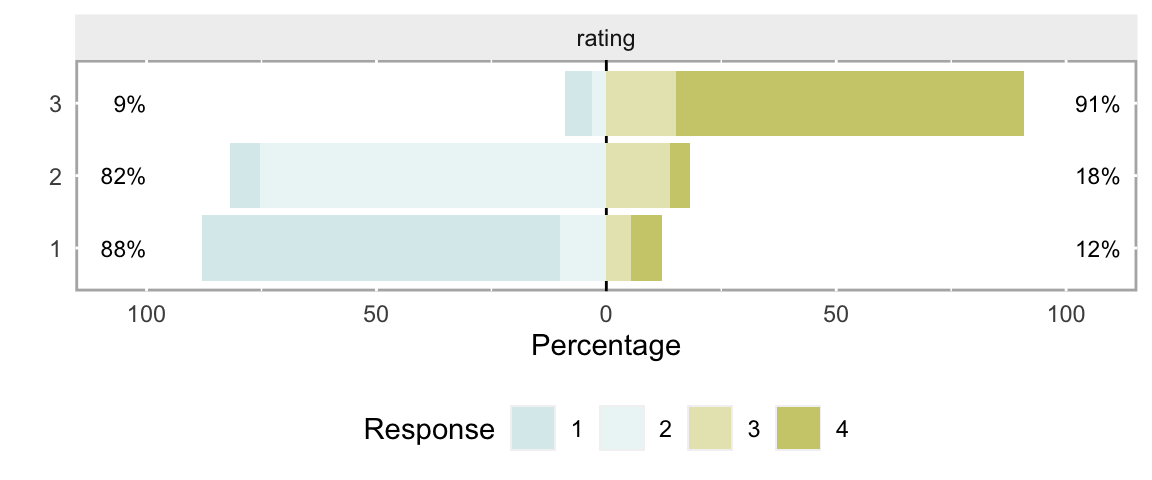
In this second scenario, the distribution of rating is specified directly as a function of group membership. This is an extreme example, designed to elicit a very high value of \(V\):
def <- defData(varname = "grp",
            formula = "0.3; 0.5; 0.2", dist = "categorical")

defc <- defCondition(condition = "grp == 1",
            formula = "0.75; 0.15; 0.05; 0.05", dist = "categorical")
defc <- defCondition(defc, condition = "grp == 2",
            formula = "0.05; 0.75; 0.15; 0.05", dist = "categorical")
defc <- defCondition(defc, condition = "grp == 3",
            formula = "0.05; 0.05; 0.15; 0.75", dist = "categorical")

# generate the data

dgrp <- genData(500, def)
dgrp <- addCondition(defc, dgrp, "rating")
It is readily apparent that the structure of the data is highly dependent on the group:
And, as expected, the estimated \(V\) is quite high:
observed <- dgrp[, table(grp, rating)]

CramerV(observed, conf.level = 0.95)
## Cramer V lwr.ci upr.ci
## 0.7400 0.6744 0.7987
Interpretation of Cramér’s V using proportional odds
A key question is how we should interpret V? Some folks suggest that \(V \le 0.10\) is very weak and anything over \(0.25\) could be considered quite strong. I decided to explore this a bit by seeing how various cumulative odds ratios relate to estimated values of \(V\).
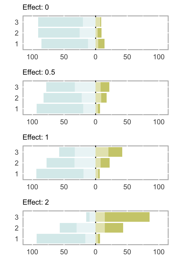
To give a sense of what some log odds ratios (LORs) look like, I have plotted distributions generated from cumulative proportional odds models, using LORs ranging from 0 to 2. At 0.5, there is slight separation between the groups, and by the time we reach 1.0, the differences are considerably more apparent:
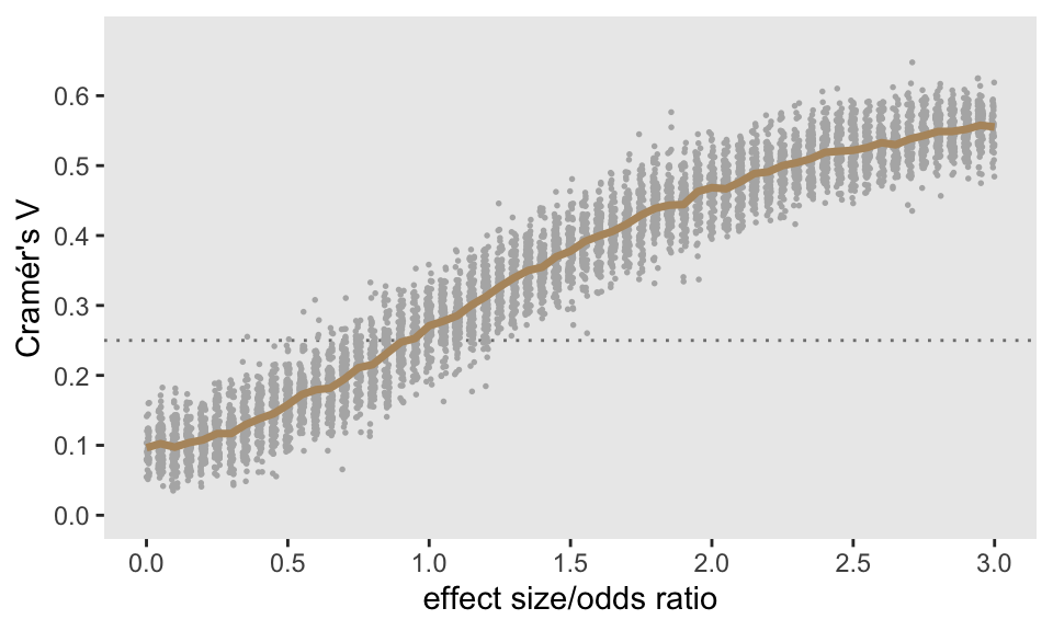
My goal was to see how estimated values of \(V\) change with the underlying LORs. I generated 100 data sets for each LOR ranging from 0 to 3 (increasing by increments of 0.05) and estimated \(V\) for each data set (of which there were 6100). The plot below shows the mean \(V\) estimate (in yellow) at each LOR, with the individual estimates represented by the grey points. I’ll let you draw you own conclusions, but (in this scenario at least), it does appear that 0.25 (the dotted horizontal line) signifies a pretty strong relationship, as LORs larger than 1.0 generally have estimates of \(V\) that exceed this threshold.
p-values and Cramér’s V
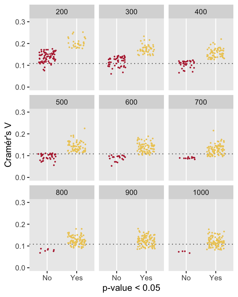
To end, I am just going to circle back to where I started at the beginning of the previous post, thinking about p-values and effect sizes. Here, I’ve generated data sets with a relatively small between-group difference, using a modest LOR of 0.40 that translates to a measure of association \(V\) just over 0.10. I varied the sample size from 200 to 1000. For each data set, I estimated \(V\) and recorded whether or not the p-value from a chi-square test would have been deemed “significant” (i.e. p-value \(< 0.05\)) or not. The key point here is that as the sample size increases and we rely solely on the chi-squared test, we are increasingly likely to attach importance to the findings even though the measure of association is quite small. However, if we actually consider a measure of association like Cramér’s \(V\) (or some other measure that you might prefer) in drawing our conclusions, we are less likely to get over-excited about a result when perhaps we shouldn’t.
I should also comment that at smaller sample sizes, we will probably over-estimate the measure of association. Here, it would be important to consider some measure of uncertainty, like a 95% confidence interval, to accompany the point estimate. Otherwise, as in the case of larger sample sizes, we would run the risk of declaring success or finding a difference when it may not be warranted.
Addendum: Why is Cramér’s V \(\le\) 1?
Cramér’s \(V = \sqrt{\frac{\chi^2/N}{min(r-1, c-1)}}\), which cannot be lower than 0. \(V=0\) when \(\chi^2 = 0\), which will only happen when the observed cell counts for all cells equal the expected cell counts for all cells. In other words, \(V=0\) only when there is complete independence.
It is also the case that \(V\) cannot exceed \(1\). I will provide some intuition for this using a relatively simple example and some algebra. Consider the following contingency table which represents complete separation of the three groups:
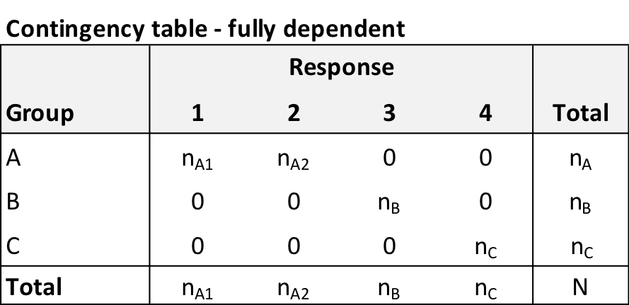
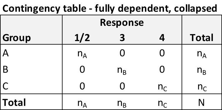
I would argue that this initial \(3 \times 4\) table is equivalent to the following \(3 \times 3\) table that collapses responses \(1\) and \(2\) - no information about the dependence has been lost or distorted. In this case \(n_A = n_{A1} + n_{A2}\).
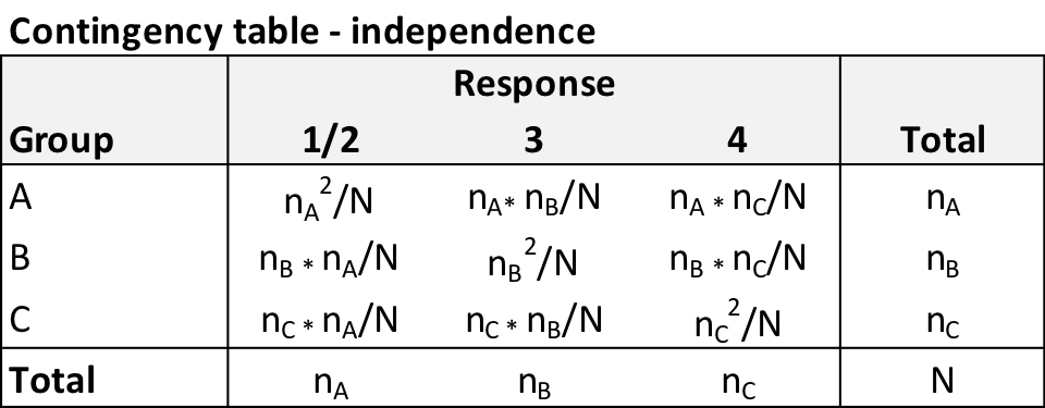
In order to calculate \(\chi^2\), we need to derive the expected values based on this collapsed contingency table. If \(p_{ij}\) is the probability for cell row \(i\) and column \(j\), and \(p_i.\) and \(p._j\) are the row \(i\) and column \(j\) totals, respectively then independence implies that \(p_{ij} = p_i.p._j\). In this example, under independence, the expected cell count for cell \(i,j\) is \(\frac{n_i}{N} \frac{n_j}{N} N = \frac{n_in_j}{N}\):
If we consider the contribution of group \(A\) to \(\chi^2\), we start with the \(\sum_{group \ A} (O_j - E_j)^2/E_j\) and end up with \(N - n_A\):
\[ \begin{aligned} \chi^2_{\text{rowA}} &= \frac{\left ( n_A - \frac{n_A^2}{N} \right )^2}{\frac{n_A^2}{N}} + \frac{\left ( \frac{n_An_B}{N} \right )^2}{\frac{n_An_B}{N}} + \frac{\left ( \frac{n_An_C}{N} \right )^2}{\frac{n_An_C}{N}} \\ \\ &= \frac{\left ( n_A - \frac{n_A^2}{N} \right )^2}{\frac{n_A^2}{N}} + \frac{n_An_B}{N}+ \frac{n_An_C}{N} \\ \\ &=N \left ( \frac{n_A^2 - \frac{2n_A^3}{N} +\frac{n_A^4}{N^2}} {n_A^2} \right ) + \frac{n_An_B}{N}+ \frac{n_An_C}{N} \\ \\ &=N \left ( 1 - \frac{2n_A}{N} +\frac{n_A^2}{N^2} \right ) + \frac{n_An_B}{N}+ \frac{n_An_C}{N} \\ \\ &= N - 2n_A +\frac{n_A^2}{N} + \frac{n_An_B}{N}+ \frac{n_An_C}{N} \\ \\ &= N - 2n_A + \frac{n_A}{N} \left ( {n_A} + n_B + n_C \right ) \\ \\ &= N - 2n_A + \frac{n_A}{N} N \\ \\ &= N - n_A \end{aligned} \]
If we repeat this on rows 2 and 3 of the table, we will find that \(\chi^2_{\text{rowB}} = N - n_B\), and \(\chi^2_{\text{rowC}} = N - n_C\), so
\[ \begin{aligned} \chi^2 &= \chi^2_\text{rowA} +\chi^2_\text{rowB}+\chi^2_\text{rowC} \\ \\ &=(N - n_A) + (N - n_B) + (N - n_C) \\ \\ &= 3N - (n_A + n_B + n_C) \\ \\ &= 3N - N \\ \\ \chi^2 &= 2N \end{aligned} \]
And
\[ \frac{\chi^2}{2 N} = 1 \]
So, under this scenario of extreme separation between groups,
\[ V = \sqrt{\frac{\chi^2}{\text{min}(r-1, c-1) \times N}} = 1 \]
where \(\text{min}(r - 1, c - 1) = \text{min}(2, 3) = 2\).