A colleague reached out for help designing a cluster randomized trial to evaluate a clinical decision support tool for primary care physicians (PCPs), which aims to improve care for high-risk patients. The outcome will be a time-to-event measure, collected at the patient level. The unit of randomization will be the PCP, and one of the key design issues is settling on the number to randomize. Surprisingly, I’ve never been involved with a study that required a clustered survival analysis. So, this particular sample size calculation is new for me, which led to the development of simulations that I can share with you. (There are some analytic solutions to this problem, but there doesn’t seem to a consensus about the best approach to use.)
Overview
In tackling this problem, there were four key elements that I needed to work out before actually conducting the power simulations. First, I needed to determine the hypothetical survival curve in the context of a single (control) arm and simulate data to confirm that I could replicate the desired curve. Second, I wanted to generate cluster-level variation so that I could assess the implications of the variance assumptions (still in a single-arm context). Third, I generated two intervention arms (without any clustering) to assess effect size assumptions. And lastly, I generated a full data set that included clustering, randomization, and censoring, and then fit a model that would be the basis for the power analysis to ensure that everything was working as expected. Once this was all completed, I was confident that I could move on to generating estimates of power under a range of sample size and variability assumptions. I apologize in advance for a post that is a bit long, but the agenda is quite packed and includes a lot of code.
Defining shape of survival curve
Defining the shape of the survival curve is made relatively easy using the function survGetParams in the simstudy package. All we need to do is specify some (at least two) coordinates along the curve and the function will return the parameters for the mean and shape of a Weibull function that best fit the points. These parameters are used in the data generation process. In this case, the study’s investigators provided me with a couple of points, indicating that approximately 10% of the sample would have an event by day 30, and half would have an event at day 365. Since the study is following patients at most for 365 days, we will consider anything beyond that to be censored (more on censoring later).
To get things started, here are the libraries needed for all the code that follows:
library(simstudy)
library(data.table)
library(survival)
library(survminer)
library(GGally)
library(coxme)
library(parallel)
Now, we get the parameters that define the survival curve:
points <- list(c(30, 0.90), c(365, .50))
r <- survGetParams(points)
r
## [1] -4.8 1.3To simulate data from this curve, the time-to-event variable tte is defined using these parameters generating by survGetParams. The observed time is the minimum of one year and the time-to-event, and we create an event indicator if the time-to-even is less than one year.
defs <- defSurv(varname = "tte", formula = r[1], shape = r[2])

defa <- defDataAdd(varname = "time", formula = "min(365, tte)", dist = "nonrandom")
defa <- defDataAdd(defa, "event", "1*(tte <= 365)", dist = "nonrandom")
Generating the data is quite simple in this case:
set.seed(589823)

dd <- genData(1000)
dd <- genSurv(dd, defs, digits = 0)
dd <- addColumns(defa, dd)

dd
## id tte time event
## 1: 1 234 234 1
## 2: 2 1190 365 0
## 3: 3 395 365 0
## 4: 4 178 178 1
## 5: 5 72 72 1
## ---
## 996: 996 818 365 0
## 997: 997 446 365 0
## 998: 998 118 118 1
## 999: 999 232 232 1
## 1000: 1000 5308 365 0The plots below show the source function determined by the parameters on the left and the actual data generated on the right. It appears that the generated data matches the data generation process:
splot <- survParamPlot(r[1], r[2], points = points, n = 1000, limits = c(0, 365) )

fit <- survfit(Surv(time, event) ~ 1, data = dd)

j <- ggsurv(fit, CI = FALSE, surv.col = "#ed7c67", size.est = 0.8) +
  theme(panel.grid = element_blank(),
        axis.text = element_text(size = 7.5),
        axis.title = element_text(size = 8, face = "bold"),
        plot.title = element_blank()) +
  ylim(0, 1) +
  xlab("time") + ylab("probability of survival")

ggarrange(splot, j, ncol = 2, nrow = 1)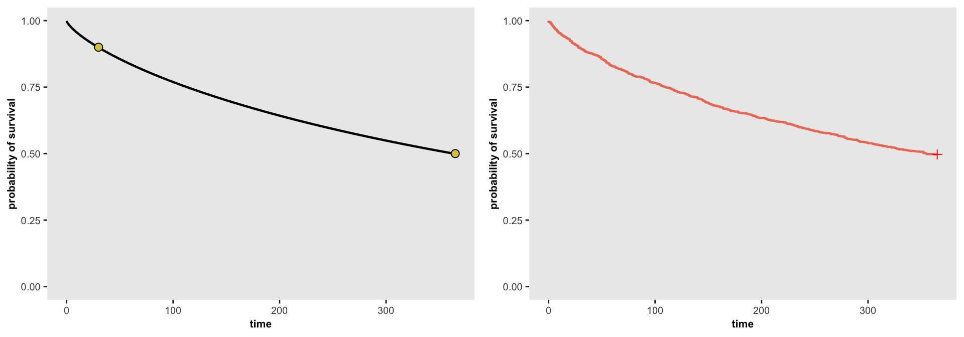
Evaluating cluster variation
Cluster variation in the context of survival curves implies that there is a cluster-specific survival curve. This variation is induced with a random effect in in the data generation process. In this case, I am assuming a normally distributed random effect with mean 0 and some variance (distributions other than a normal distribution can be used). The variance assumption is a key one (which will ultimately impact the estimates of power), and I explore that a bit more in the second part of this section.
Visualizing cluster variation
The data generation process is a tad more involved than above, though not much more. We need to generate clusters and their random effect first, before adding the individuals. tte is now a function of the distribution parameters as well as the cluster random effect b. We are still using a single arm and assuming that everyone is followed for one year. In the first simulation, we set the random effect variance \(b = 0.1\).
defc <- defData(varname = "b", formula = 0, variance = 0.1)

defs <- defSurv(varname = "tte", formula = "r[1] + b", shape = r[2])

defa <- defDataAdd(varname = "time", formula = "min(365, tte)", dist = "nonrandom")
defa <- defDataAdd(defa, "event", "1*(tte <= 365)", dist = "nonrandom")
dc <- genData(20, defc, id = "pcp")
dd <- genCluster(dc, "pcp", numIndsVar = 1000, "id")
dd <- genSurv(dd, defs, digits = 0)
dd.10 <- addColumns(defa, dd)
dd.10## pcp b id tte time event
## 1: 1 0.25 1 788 365 0
## 2: 1 0.25 2 93 93 1
## 3: 1 0.25 3 723 365 0
## 4: 1 0.25 4 151 151 1
## 5: 1 0.25 5 1367 365 0
## ---
## 19996: 20 0.22 19996 424 365 0
## 19997: 20 0.22 19997 207 207 1
## 19998: 20 0.22 19998 70 70 1
## 19999: 20 0.22 19999 669 365 0
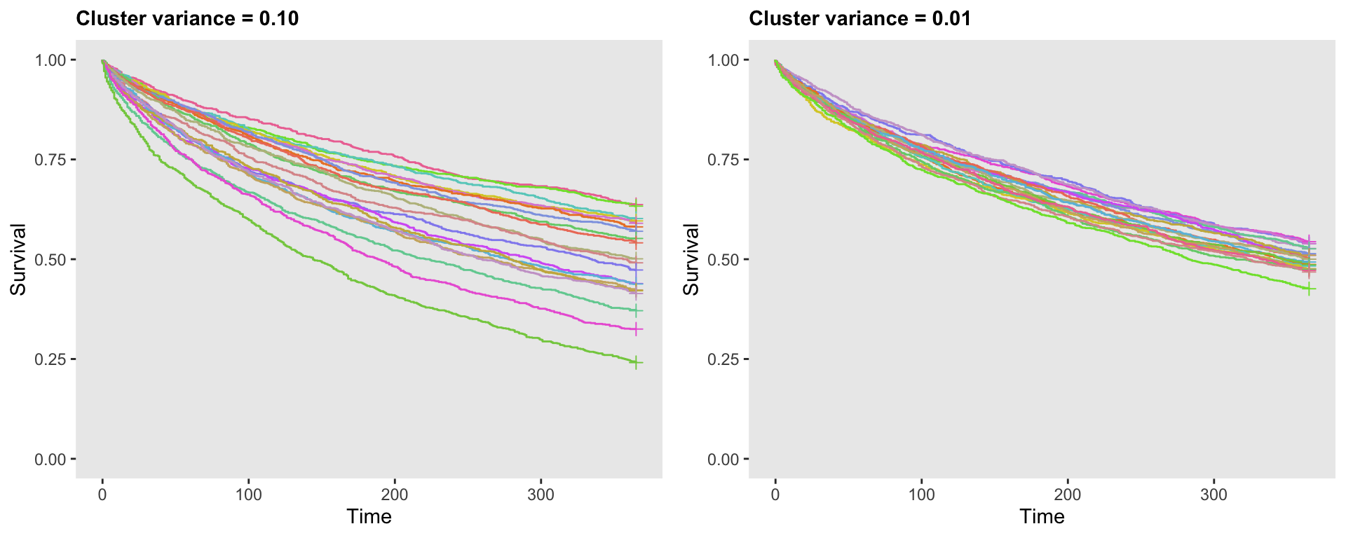
## 20000: 20 0.22 20000 994 365 0The following plot shows two sets of survival curves, each based on different levels of variation, 0.10 on the left, and 0.01 on the right. Each curve represents a different cluster. With this plot, we get a clear visualization of how variance assumption of the random effect impacts the variation of the survival curves:
Variation of the probability of an event across clusters
The plot of the survival curves is only one way to consider the impact of cluster variation. Another option is to look at the binary event outcome under the assumption of no censoring. I like to evaluate the variation in the probability of an event across the clusters, particularly by looking at the range of probabilities, or considering the coefficient of variation, which is \(\sigma / \mu\).
To show how this is done, I am generating a data set with a very large number of clusters (2000) and a large cluster size (500), and then calculating the probability of an event for each cluster:
defc <- defData(varname = "b", formula = 0, variance = 0.100)

dc <- genData(2000, defc, id = "pcp")
dd <- genCluster(dc, "pcp", numIndsVar = 500, "id")
dd <- genSurv(dd, defs, digits = 0)
dd <- addColumns(defa, dd)

ds <- dd[, .(p = mean(event)), keyby = pcp]
ds
## pcp p
## 1: 1 0.41
## 2: 2 0.43
## 3: 3 0.36
## 4: 4 0.51
## 5: 5 0.50
## ---
## 1996: 1996 0.82
## 1997: 1997 0.53
## 1998: 1998 0.88
## 1999: 1999 0.42
## 2000: 2000 0.63Here is the distribution of observed cluster-level proportions:
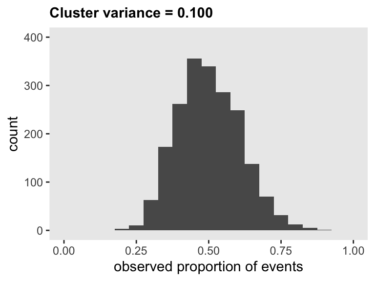
Here are the mean probability, the standard deviation of probabilities, the coefficient of variation for the probabilities, and the 95% interval of the probabilities when the random effect variance in the survival generation process is 0.10:
ds[, .(mu = mean(p), s = sd(p), cv = sd(p)/mean(p))]## mu s cv
## 1: 0.5 0.11 0.22ds[, .(quantile(p, probs = c(0.025, .975)))]## V1
## 1: 0.31
## 2: 0.72To compare across a range variance assumptions, I’ve generated ten data sets and plotted the results below. If you hover over the points, you will get the CV estimate. This could be helpful in helping collaborators decide what levels of variance is appropriate to focus on in the final power estimation and sample size determination.
In this case, we’ve decided that a coefficient of variation is not likely to exceed 0.17 (with a corresponding 95% interval of proportions ranging from 35% to 66%), so we’ll consider that when evaluating power.
Evaluating the effect size
Next, we generate data that includes treatment assignment (but excludes cluster variability and censoring before one year). The treatment effect is expressed as a log hazard ratio, which in this case 0.4 (equal to a hazard ratio of just about 1.5).
The data generation starts with treatment assignment, adds the time-to-event survival data, and then adds the one-year censoring data, as before:
defa <- defData(varname = "rx", formula = "1;1", dist = "trtAssign")

defs <- defSurv(varname = "tte", formula = "r[1] + 0.4 * rx", shape = r[2])

defe <- defDataAdd(varname = "time", formula = "min(365, tte)", dist = "nonrandom")
defe <- defDataAdd(defe, "event", "1*(tte <= 365)", dist = "nonrandom")

dd <- genData(1000, defa)
dd <- genSurv(dd, defs, digits = 0)
dd <- addColumns(defe, dd)

dd
## id rx tte time event
## 1: 1 0 1902 365 0
## 2: 2 0 286 286 1
## 3: 3 0 480 365 0
## 4: 4 0 32 32 1
## 5: 5 1 12 12 1
## ---
## 996: 996 0 663 365 0
## 997: 997 1 962 365 0
## 998: 998 1 19 19 1
## 999: 999 1 502 365 0
## 1000: 1000 0 85 85 1The plot of the survival curves by treatment arms provides a visualization of the treatment effect:
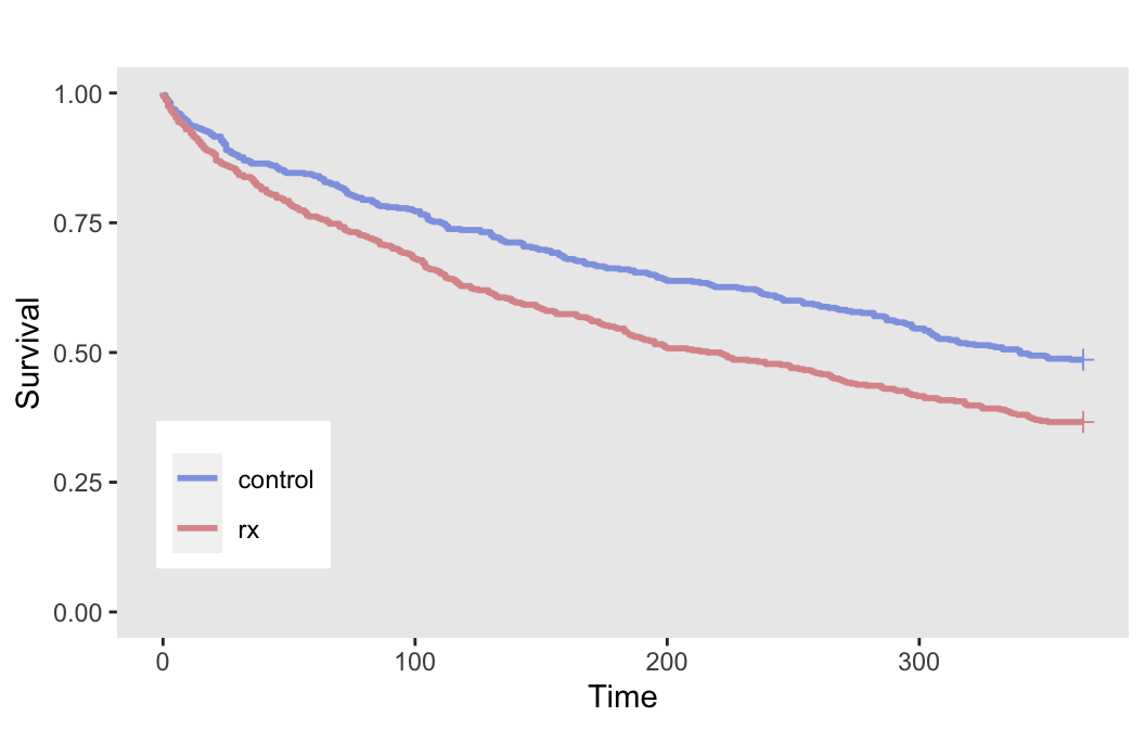
Again, since we have no censoring, we can estimate the probability of an event within 365 days for each arm:
dd[, .(p = mean(event)), keyby = rx]## rx p
## 1: control 0.51
## 2: rx 0.63An effect size of 0.4 on the log hazard scale translates to an odds ratio of about 1.64, a risk ratio of 1.24, and risk difference of 12 percentage points. In the absence of any external data on the potential effect size, we can use an effect size that is minimally clinically meaningful based on any or all these effect size measurements.
Complete data generation and model estimation
With the pieces in place, we are ready to put it all together and add censoring to the mix to finalize the full data generating process. We will fit a mixed-effects Cox proportional hazards model to see if we can recover the parameters that we have used to generate the data, and, if that goes well, we will be ready to estimate power.
We start in defc by defining the cluster-level random effect variation and treatment assignment design (in this case 1 to 1, treatment to control). We add a censoring process in defa. This assumes that we will be enrolling patients for six months, spread out across this time period. The study will last exactly one year, so every patient will be followed for at least six months, and only some will be followed for a full year (i.e., those who join the study on the first day).
Finally, defs defines the data generation process for the survival outcome, which we’ve seen above, though now we have both a treatment effect and a random effect, in addition to the baseline parameters in the vector r.
defc <- defData(varname = "b", formula = 0, variance = 0.05)
defc <- defData(defc, varname = "rx", formula = "1;1", dist = "trtAssign")

defa <- defDataAdd(varname = "start_day", formula = "1;182", dist = "uniformInt")
defa <- defDataAdd(defa, varname = "censor",
  formula = "365 - start_day ", dist = "nonrandom")

defs <- defSurv(varname = "tte", formula = "r[1] + 0.4 * rx + b", shape = r[2])
The data generation is the same as before, though there is an additional censoring process, which is done with the function addCompRisk:
dc <- genData(500, defc, id = "pcp")
dd <- genCluster(dc, "pcp", numIndsVar = 200, "id")
dd <- addColumns(defa, dd)
dd <- genSurv(dd, defs, digits = 0)
dd <- addCompRisk(dd, events = c("tte", "censor"),
  timeName = "time", censorName = "censor", keepEvents = TRUE)

dd
## pcp b rx id start_day censor tte time event type
## 1: 1 -0.0158 1 1 65 300 307 300 0 censor
## 2: 1 -0.0158 1 2 113 252 907 252 0 censor
## 3: 1 -0.0158 1 3 121 244 110 110 1 tte
## 4: 1 -0.0158 1 4 60 305 170 170 1 tte
## 5: 1 -0.0158 1 5 95 270 2673 270 0 censor
## ---
## 99996: 500 -0.0015 0 99996 160 205 291 205 0 censor
## 99997: 500 -0.0015 0 99997 79 286 193 193 1 tte
## 99998: 500 -0.0015 0 99998 64 301 28 28 1 tte
## 99999: 500 -0.0015 0 99999 153 212 459 212 0 censor
## 100000: 500 -0.0015 0 100000 19 346 298 298 1 tteSince we have generated a rather large data set, we should be able to recover the parameters pretty closely if we are using the correct model. We are going to fit a mixed effects survival model (also known as a frailty model) to see how well we did.
fit_coxme <- coxme(Surv(time, event) ~ rx + (1 | pcp), data = dd)
summary(fit_coxme)
## Cox mixed-effects model fit by maximum likelihood
## Data: dd
## events, n = 49955, 1e+05
## Iterations= 11 48
## NULL Integrated Fitted
## Log-likelihood -555429 -553708 -553058
##
## Chisq df p AIC BIC
## Integrated loglik 3442 2 0 3438 3421
## Penalized loglik 4743 414 0 3914 259
##
## Model: Surv(time, event) ~ rx + (1 | pcp)
## Fixed coefficients
## coef exp(coef) se(coef) z p
## rx 0.39 1.5 0.022 18 0
##
## Random effects
## Group Variable Std Dev Variance
## pcp Intercept 0.22 0.05Pretty good! The estimated HR of 0.39 (95% CI: 0.35 - 0.43) is on target (we used 0.40 in the data generation process), and the estimated variance for the PCP random effect was 0.05, also on the mark. I’d say we are ready to proceed to the final step.
Power estimation
To conduct the power estimation, I’ve essentially wrapped the data generation and model estimation code in a collection of functions that can be called repeatedly to generate multiple data sets and model estimates The goal is to calculate the proportion of data sets with a statistically significant result for a particular set of assumptions (i.e., the estimate of power for the assumed effect size, variation, and sample sizes). I’ve provided the code below in the addendum in case you haven’t grown weary of all this detail. I described a general framework for using simulation to estimate sample size/power, and I’m largely following that process here.
I’ve written a little function scenario_list (which I’m now thinking I should add to simstudy) to create different parameter combinations that will determine the power estimation. In this case, the parameters I am interested in are the number of PCPs that should be randomized and the variance assumption. The number of patients per PCP (cluster size) is also important to vary, but for illustration purposes here I am keeping it constant.
Here is the simplified scenario list with four possible combinations:
scenario_list <- function(...) {
  argmat <- expand.grid(...)
  return(asplit(argmat, MARGIN = 1))
}

npcps <- c(20, 30)
npats <- c(15)
s2 <- c(0.03, 0.04)

scenarios <- scenario_list(npcps = npcps, npats = npats, s2 = s2)

scenarios
## [[1]]
## npcps npats s2
## 20.00 15.00 0.03
##
## [[2]]
## npcps npats s2
## 30.00 15.00 0.03
##
## [[3]]
## npcps npats s2
## 20.00 15.00 0.04
##
## [[4]]
## npcps npats s2
## 30.00 15.00 0.04I use the mclapply function in the parallel package to generate three iterations for each scenario:
model.ests <- mclapply(scenarios, function(a) s_scenarios(a, nrep = 3))

model.ests
## [[1]]
## npcps npats s2 est_s re.var_s p_s
## 1: 20 15 0.03 0.41 0.1596 0.100
## 2: 20 15 0.03 0.32 0.0306 0.065
## 3: 20 15 0.03 0.32 0.0004 0.041
##
## [[2]]
## npcps npats s2 est_s re.var_s p_s
## 1: 30 15 0.03 0.13 0.017 3.5e-01
## 2: 30 15 0.03 0.62 0.029 7.3e-05
## 3: 30 15 0.03 0.45 0.040 3.8e-03
##
## [[3]]
## npcps npats s2 est_s re.var_s p_s
## 1: 20 15 0.04 0.55 7.9e-02 0.0084
## 2: 20 15 0.04 0.07 4.0e-04 0.6700
## 3: 20 15 0.04 0.24 8.2e-05 0.1500
##
## [[4]]
## npcps npats s2 est_s re.var_s p_s
## 1: 30 15 0.04 0.42 8.3e-05 2.7e-03
## 2: 30 15 0.04 0.57 4.0e-04 2.6e-05
## 3: 30 15 0.04 0.36 1.0e-01 4.2e-02In the actual power calculations, which are reported below, I used 60 scenarios defined by these data generation parameters:
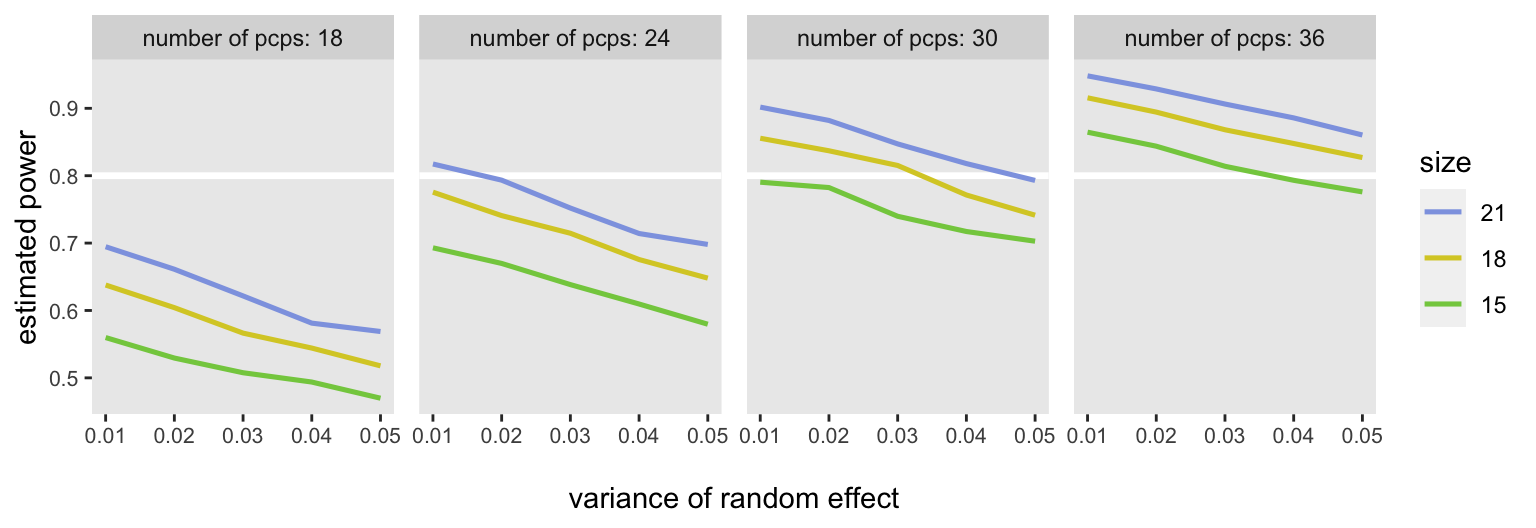
npcps <- c(18, 24, 30, 36)
npats <- c(15, 18, 21)
s2 <- c(0.01, 0.02, 0.03, 0.04, 0.05)
For each of these scenarios, I generated 5000 data sets and estimated models for each (i.e., a total of 300,000 data sets and model fits). For each of the 60 scenarios, I estimated the proportion of the 5000 model fits that yielded a p-value < 0.05 for the estimated log hazard ratio. I had the benefit of using a high performance computer, because running this on my laptop would have taken well over 10 hours (only about 10 minutes on the HPC).
At the end, we have a plot of “power curves” that shows estimated power for each of the scenarios. If we assume that we can expect at least 18 patients per PCP and that the between-PCP variance will be around 0,03 or 0.04, we should be OK randomizing 30 PCPs (15 in each arm), though it might more prudent to go with 36, just to be safe:
Addendum
Here is the code I used to generate the data for the power curve plot. It is based on the framework I mentioned earlier. There is one extra function here, extract_coxme_table, which I pulled from stackoverflow, because there is currently no obvious way to extract data from the coxme model fit.
extract_coxme_table <- function (mod) {
  beta <- mod$coefficients
  nvar <- length(beta)
  nfrail <- nrow(mod$var) - nvar
  se <- sqrt(diag(mod$var)[nfrail + 1:nvar])
  z <- round(beta/se, 2)
  p <- signif(1 - pchisq((beta/se)^2, 1), 2)
  table=data.table(beta = beta, se = se, z = z, p = p)
  return(table)
}

s_def <- function() {

  defc <- defData(varname = "b", formula = 0, variance = "..s2")
  defc <- defData(defc, varname = "rx", formula = "1;1", dist = "trtAssign")

  defa <- defDataAdd(varname = "start_day", formula = "1;182", dist = "uniformInt")
  defa <- defDataAdd(defa, varname = "censor",
                     formula = "365 - start_day ", dist = "nonrandom")

  defs <- defSurv(varname = "tte", formula = "-4.815 + 0.4 * rx + b", shape = 1.326)

  defa2 <- defDataAdd(varname = "event6",
                      formula = "1*(tte <= 182)", dist = "nonrandom")

  return(list(defc = defc, defa = defa, defs = defs, defa2 = defa2))

}

s_generate <- function(argsvec, list_of_defs) {

  list2env(list_of_defs, envir = environment())
  list2env(as.list(argsvec), envir = environment())

  dc <- genData(npcps, defc, id = "pcp")
  dd <- genCluster(dc, "pcp", npats, "id")
  dd <- addColumns(defa, dd)
  dd <- genSurv(dd, defs, digits = 0)
  dx <- addCompRisk(dd, events = c("tte", "censor"),
                    timeName = "time", censorName = "censor", keepEvents = TRUE)
  dx <- addColumns(defa2, dx)

  dx[]

}

s_replicate <- function(argsvec, list_of_defs) {

  dx <- s_generate(argsvec, list_of_defs)

  coxfitm <-coxme(Surv(time, event) ~ rx + (1 | pcp), data = dx)

  list2env(as.list(argsvec), envir = environment())

  return(data.table(
    npcps = npcps,
    npats = npats,
    s2 = s2,
    est_s = fixef(coxfitm),
    re.var_s = VarCorr(coxfitm)$pcp,
    p_s = extract_coxme_table(coxfitm)$p
  ))

}

s_scenarios <- function(argsvec, nreps) {

  list_of_defs <- s_def()

  rbindlist(
    parallel::mclapply(
      X = 1 : nreps,
      FUN = function(x) s_replicate(argsvec, list_of_defs),
      mc.cores = 4)
  )

}