Framework for power analysis using simulation

The framework

I will provide a simple application below, but first I’ll show the general structure. The basic idea is that we want to generate data under a variety of assumptions - for example, a power analysis will assume different sample sizes, effects, and/or levels of variation - and for each set of assumptions, we want to generate a large number of replications to mimic repeated sampling from a population. The key elements of the process include (1) defining the data, (2) generating a data set, (3) fitting a model to the data, and (4) providing summary statistics.

If you have familiarity with simstudy, I’d say the code is pretty self-explanatory. In the function s_generate, there is a call to base R function list2env, which makes all elements of a list available as variables in the function’s environment. The replication process is managed by the mclapply function from the parallel package. (Alternative approaches include using function lapply in base R or using a for loop.)

s_define <- function() {
  
  #--- add data definition code ---#
  
  return(list_of_defs) # list_of_defs is a list of simstudy data definitions
}

s_generate <- function(list_of_defs, argsvec) {
  
  list2env(list_of_defs, envir = environment())
  list2env(as.list(argsvec), envir = environment())
  
  #--- add data generation code ---#
  
  return(generated_data) #  generated_data is a data.table
}

s_model <- function(generated_data) {
  
  #--- add model code ---#
  
  return(model_results) # model_results is a data.table
}

s_single_rep <- function(list_of_defs, argsvec) {
  
  generated_data <- s_generate(list_of_defs, argsvec)
  model_results <- s_model(generated_data)
  
  return(model_results)
}

s_replicate <- function(argsvec, nsim) {
  
  list_of_defs <- s_define()

  model_results <- rbindlist(
    parallel::mclapply(
      X = 1 : nsim, 
      FUN = function(x) s_single_rep(list_of_defs, argsvec), 
      mc.cores = 4)
  )
  
  #--- add summary statistics code ---#
  
  return(summary_stats) # summary_stats is a data.table
}

#---- specify varying power-related parameters ---#

scenario_list <- function(...) {
  argmat <- expand.grid(...)
  return(asplit(argmat, MARGIN = 1))
}

param_1 <- c(...)
param_2 <- c(...)
param_3 <- c(...)
.
.
.

scenarios <- scenario_list(param1 = param_1, param_2 = param_2, param_3 = param_3, ...)

#--- run locally ---#

summary_stats <- rbindlist(lapply(scenarios, function(a) s_replicate(a, nsim = 1000)))

Example: power analysis of a CRT

To carry out a power analysis of a cluster randomized trial, I’ll fill in the skeletal framework. In this case I am interested in understanding how estimates of power vary based on changes in effect size, between cluster/site variation, and the number of patients per site. The data definitions use double dot notation to allow the definitions to change dynamically as we switch from one scenario to the next. We estimate a mixed effect model for each data set and keep track of the proportion of p-value estimates less than 0.05 for each scenario.

s_define <- function() {
  
  #--- data definition code ---#
  
  def1 <- defData(varname = "site_eff", 
    formula = 0, variance = "..svar", dist = "normal", id = "site")
  def1 <- defData(def1, "npat", formula = "..npat", dist = "poisson")
  
  def2 <- defDataAdd(varname = "Y", formula = "5 + site_eff + ..delta * rx", 
    variance = 3, dist = "normal")
  
  return(list(def1 = def1, def2 = def2)) 
}

s_generate <- function(list_of_defs, argsvec) {
  
  list2env(list_of_defs, envir = environment())
  list2env(as.list(argsvec), envir = environment())
  
  #--- data generation code ---#
  
  ds <- genData(40, def1)
  ds <- trtAssign(ds, grpName = "rx")
  dd <- genCluster(ds, "site", "npat", "id")
  dd <- addColumns(def2, dd)
  
  return(dd)
}

s_model <- function(generated_data) {
  
  #--- model code ---#
  
  require(lme4)
  require(lmerTest)
  
  lmefit <- lmer(Y ~ rx + (1|site), data = generated_data)
  est <- summary(lmefit)$coef[2, "Estimate"]
  pval <- summary(lmefit)$coef[2, "Pr(>|t|)"]
  
  return(data.table(est, pval)) # model_results is a data.table
}

s_single_rep <- function(list_of_defs, argsvec) {
  
  generated_data <- s_generate(list_of_defs, argsvec)
  model_results <- s_model(generated_data)
  
  return(model_results)
}

s_replicate <- function(argsvec, nsim) {
  
  list_of_defs <- s_define()

  model_results <- rbindlist(
    parallel::mclapply(
      X = 1 : nsim, 
      FUN = function(x) s_single_rep(list_of_defs, argsvec), 
      mc.cores = 4)
  )
  
  #--- summary statistics ---#
  
  power <- model_results[, mean(pval <= 0.05)]
  summary_stats <- data.table(t(argsvec), power)
  
  return(summary_stats) # summary_stats is a data.table
}

scenario_list <- function(...) {
  argmat <- expand.grid(...)
  return(asplit(argmat, MARGIN = 1))
}

delta <- c(0.50, 0.75, 1.00)
svar <- c(0.25, 0.50)
npat <- c(8, 16)

scenarios <- scenario_list(delta = delta, svar = svar, npat = npat)

#--- run locally ---#

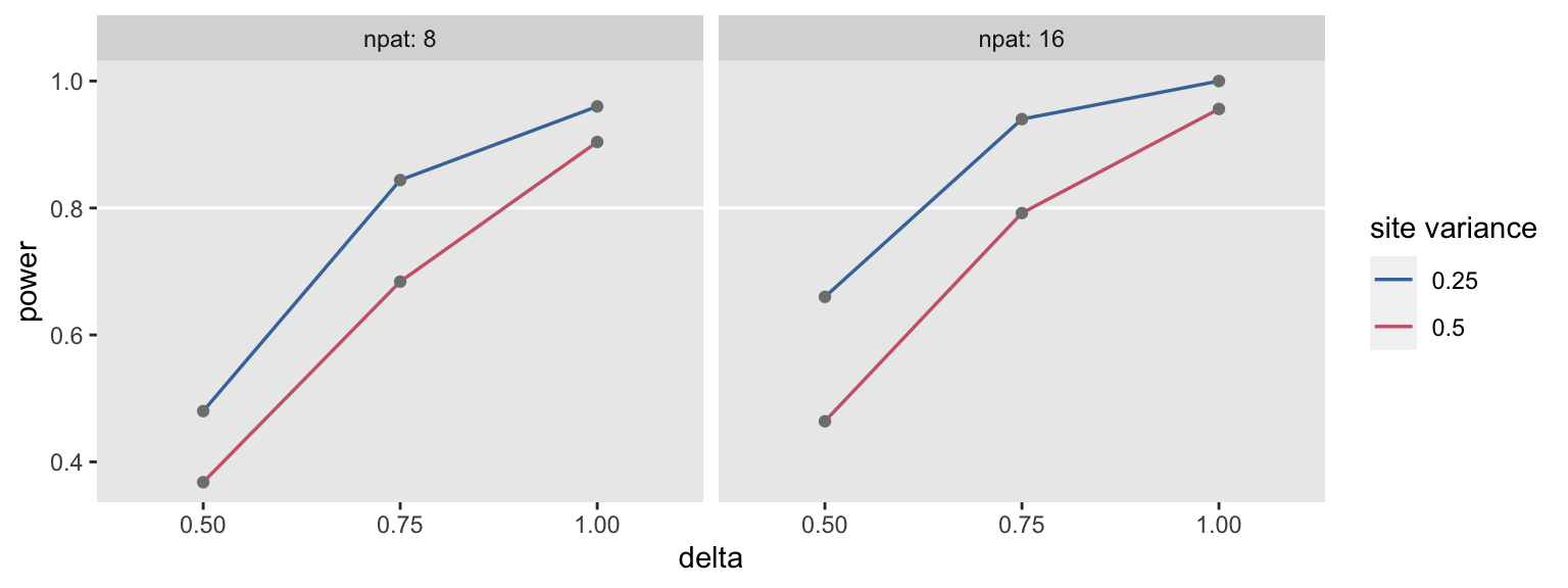
summary_stats <- rbindlist(lapply(scenarios, function(a) s_replicate(a, nsim = 250)))

The overall results (in this case, the power estimate) can be reported for each scenario.

summary_stats

##     delta svar npat power
##  1:  0.50 0.25    8 0.480
##  2:  0.75 0.25    8 0.844
##  3:  1.00 0.25    8 0.960
##  4:  0.50 0.50    8 0.368
##  5:  0.75 0.50    8 0.684
##  6:  1.00 0.50    8 0.904
##  7:  0.50 0.25   16 0.660
##  8:  0.75 0.25   16 0.940
##  9:  1.00 0.25   16 1.000
## 10:  0.50 0.50   16 0.464
## 11:  0.75 0.50   16 0.792
## 12:  1.00 0.50   16 0.956

We can also plot the results easily to get a clearer picture. Higher between-site variation clearly reduces power, as do smaller effect sizes and smaller sizes. None of this is surprising, but is always nice to see things working out as expected: