Recently I started a discussion about modeling secular trends using flexible models in the context of cluster randomized trials. I’ve been motivated by a trial I am involved with that is using a stepped-wedge study design. The initial post focused on more standard parallel designs; here, I want to extend the discussion explicitly to the stepped-wedge design.
The stepped-wedge design
Stepped-wedge designs are a special class of cluster randomized trial where each cluster is observed in both treatment arms (as opposed to the classic parallel design where only some of the clusters receive the treatment). In what is essentially a cross-over design, each cluster transitions in a single direction from control (or pre-intervention) to intervention. I’ve written about this in a number of different contexts (for example, with respect to power analysis, complicated ICC patterns, using Bayesian models for estimation, open cohorts, and baseline measurements to improve efficiency).
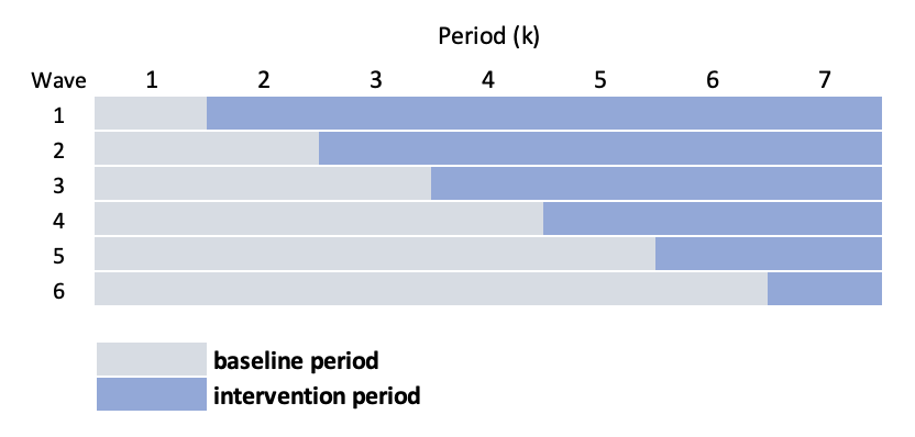
In the classic stepped-wedge design, groups of sites (considered waves) are randomized to intervention starting times. For example, if there are 24 sites divided into 6 waves (so 4 sites per wave), there will be six starting times and 7 measurement periods (if we want to have at least one baseline/control period for each wave, and at least one intervention period per wave). Schematically, the design looks like this:
We could use a linear mixed effects model to estimate the intervention effect \(\delta\), which might look like this:
\[ Y_{ijk} = a_{j} + \beta_{k} + \delta A_{jk} + e_{ijk} \]
where \(Y_{ijk}\) is the (continuous) outcome of individual \(i\) in cluster \(j\) during time period \(k\). \(a_j\) is the random intercept for site \(j\), and we assume that \(a_j \sim N(0, \sigma^2_a)\). \(A_{jk}\) is the intervention indicator for site \(j\) during time period \(k\). \(\beta_k\) is a period-specific effect. And \(e_{ijk}\) is the individual level effect, \(e_{ijk} \sim N(0, \sigma^2_e)\).
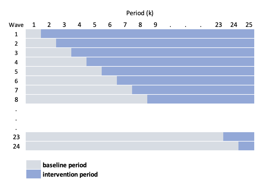
In the particular study motivating these posts, the situation is different in a key way: given its complexity, the intervention can only be implemented at one site a time, so that the number of waves equals the number of sites. This leads to this slightly more elaborate schematic:
The challenge under this scenario is that \(k\) (the number of periods) is starting to get quite large, requiring us to estimate a large number of period specific effects \(\beta_k\). In addition, the periods are actually shorter, so we have less information available to estimate those period effects. An alternative approach, as you may have anticipated, is to smooth the secular trend, using a model that looks like this:
\[ Y_{ijk} = a_{j} + s(k) + \delta A_{jk} + e_{ijk} \]
where \(s(.)\) is a smooth function of time. And by using a smooth function, we can take this one step further and specify a site-specific smoothing function \(s_j(.)\):
\[ Y_{ijk} = a_{j} + s_j(k) + \delta A_{jk} + e_{ijk} \]
So, we will use either cubic splines or generalized additive models (GAMs) to estimate the curve, which will allow us to control for the period effect while estimating the treatment effect. By smoothing the function, we are assuming that the measurements closer in time are more highly correlated than measurements further apart.
Data generation process
Here is the data generation process that we will use to explore the different models:
\[ Y_{ijk} \sim N(\mu_{ijk}, \sigma^2 = 40) \\ \mu_{ijk} = a_{j} + b_{jk} + \delta A_{jk} \\ a_j \sim N(0, \sigma^2_a = 9) \\ b_{jk} \sim N(0, \Sigma_b) \\ \delta = 5\\ \]
In this data generation process, the time effect will not be explicitly smooth, but the underlying covariance structure used to generate the period effects will induce some level of smoothness. This is similar to what was described in the previous post. As in that earlier example, \(b_{jk}\) is a site-specific time period effect for each time period \(k\); the vector of cluster-time effects \(\mathbf{b_j} \sim N(0, \Sigma_b)\), where \(\Sigma_b = DRD\) is a \(25 \times 25\) covariance matrix based on a diagonal matrix \(D\) and an auto-regressive correlation structure \(R\):
\[ D = 4 * I_{25 \times 25} \]
and
\[ R =\begin{bmatrix} 1 & \rho & \rho^2 & \dots & \rho^{24} \\ \rho & 1 & \rho & \dots & \rho^{23} \\ \rho^2 & \rho & 1 & \dots & \rho^{22} \\ \vdots & \vdots & \vdots & \vdots & \vdots \\ \rho^{24} & \rho^{23} & \rho^{22} & \dots & 1 \\ \end{bmatrix}, \ \ \rho = 0.7 \]
Now we are ready to implement this data generating process using simstudy. First the R packages that we will need:
library(simstudy)
library(ggplot2)
library(data.table)
library(mgcv)
library(lme4)
library(splines)
The data definitions for \(a_j\), \(b_{jk}\), and \(Y_{ijk}\) are established first:
def <- defData(varname = "a", formula = 0, variance = 9)
def <- defData(def, varname = "mu_b", formula = 0, dist = "nonrandom")
def <- defData(def, varname = "s2_b", formula = 16, dist = "nonrandom")

defOut <- defDataAdd(varname = "y", formula = "a + b + 5 * A", variance = 40)
We (1) generate 24 sites with random intercepts, (2) create 25 periods for each site, (3) generate the period-specific effects (\(b_{jk}\)) for each site, and (4) assign the treatment status based on the stepped-wedge design:
set.seed(1234)

ds <- genData(24, def, id = "site")                  #1
ds <- addPeriods(ds, 25, "site", perName = "k")      #2

ds <- addCorGen(dtOld = ds, idvar = "site",
                rho = 0.8, corstr = "ar1",
                dist = "normal", param1 = "mu_b",
                param2 = "s2_b", cnames = "b")       #3

ds <- trtStepWedge(ds, "site", nWaves = 24,
                   lenWaves = 1, startPer = 1,
                   grpName = "A", perName = "k")     #4

ds$site <- as.factor(ds$site)

ds
## site k a mu_b s2_b timeID b startTrt A
## 1: 1 0 -3.621197 0 16 1 -3.6889733 1 0
## 2: 1 1 -3.621197 0 16 2 -1.6620662 1 1
## 3: 1 2 -3.621197 0 16 3 1.5816344 1 1
## 4: 1 3 -3.621197 0 16 4 4.0869655 1 1
## 5: 1 4 -3.621197 0 16 5 1.9385573 1 1
## ---
## 596: 24 20 1.378768 0 16 596 -1.5470625 24 0
## 597: 24 21 1.378768 0 16 597 -1.7687554 24 0
## 598: 24 22 1.378768 0 16 598 4.1179282 24 0
## 599: 24 23 1.378768 0 16 599 7.1421562 24 0
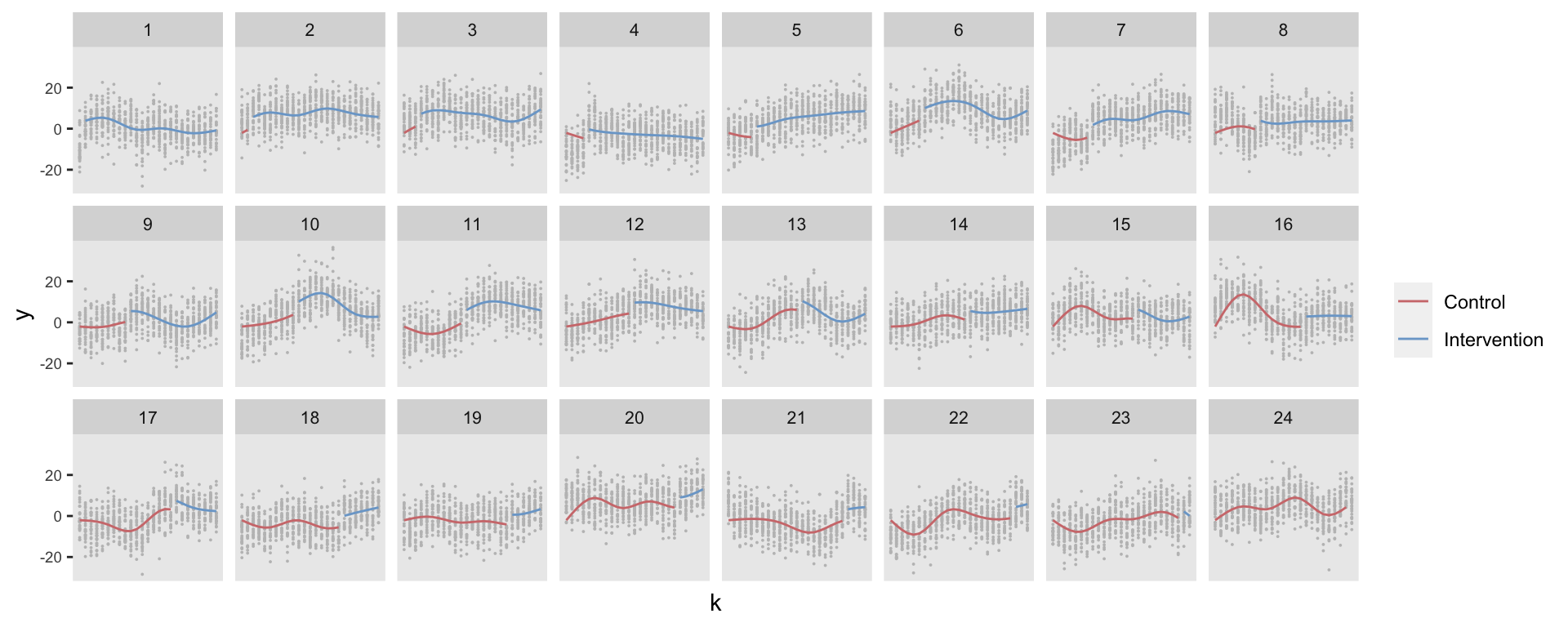
## 600: 24 24 1.378768 0 16 600 0.3645013 24 1In the last two steps, we create 30 individuals per site per period and generate each individual-level outcome. The figure shows the outcomes for all the sites over time:
dd <- genCluster(ds, "timeID", numIndsVar = 30, level1ID = "id")
dd <- addColumns(defOut, dd)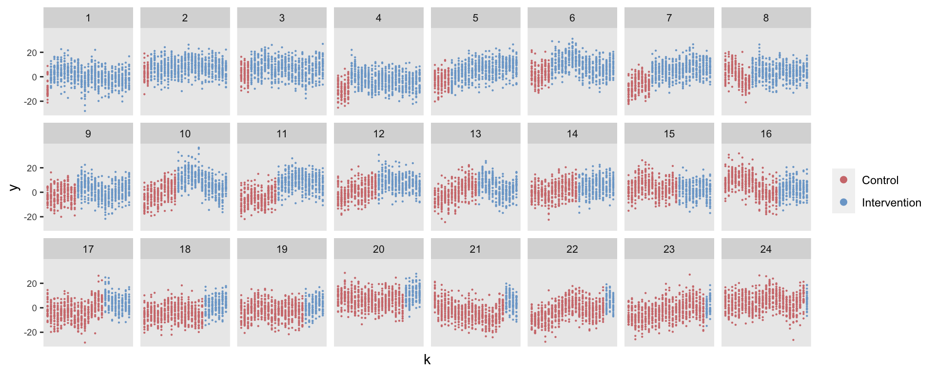
Model estimation
I am fitting three models to this simulated data set: (1) a mixed effects model with fixed time period effects, (2), a mixed effects model with a random cubic spline for the period effect for each site, and (3) a generalized additive model with a site-specific smooth function for time. For each estimated model, I’ve overlaid the predicted values on top of the observed (generated) data points.
I’ve also conducted an experiment using 5000+ replicated data sets to see how each model really performs with respect to the estimation of the treatment effect. (Code for these replications can be found here). These replications provide information about some operating characteristics of the different models (estimated bias, root mean squared error (RMSE), average estimated standard error, and coverage rate, i.e. proportion of 95% confidence intervals that include the true value 5).
Mixed effects model with fixed time-period effects
Here’s the first model. Note that I am not estimating an intercept so that each period effect is directly estimated. (I did try to estimate the 600 site-specific period random effects, but it proved too computationally intensive for my computer, which ground away for a half hour before I mercifully stopped it). The model does include a site-specific random intercept.
fitlme_k <- lmer(y ~ A + factor(k) - 1 + (1|site), data = dd)
summary(fitlme_k)
## Linear mixed model fit by REML ['lmerMod']
## Formula: y ~ A + factor(k) - 1 + (1 | site)
## Data: dd
##
## REML criterion at convergence: 122095.4
##
## Scaled residuals:
## Min 1Q Median 3Q Max
## -4.1545 -0.6781 -0.0090 0.6765 4.2816
##
## Random effects:
## Groups Name Variance Std.Dev.
## site (Intercept) 10.76 3.280
## Residual 51.37 7.167
## Number of obs: 18000, groups: site, 24
##
## Fixed effects:
## Estimate Std. Error t value
## A 5.83701 0.18482 31.582
## factor(k)0 -1.72745 0.72085 -2.396
## factor(k)1 -2.44884 0.72089 -3.397
## factor(k)2 -1.61074 0.72102 -2.234
## factor(k)3 -0.09524 0.72122 -0.132
## factor(k)4 -0.85081 0.72151 -1.179
## factor(k)5 -0.11645 0.72188 -0.161
## factor(k)6 -0.57468 0.72233 -0.796
## factor(k)7 -0.13628 0.72287 -0.189
## factor(k)8 0.01035 0.72348 0.014
## factor(k)9 -0.63440 0.72418 -0.876
## factor(k)10 0.33878 0.72496 0.467
## factor(k)11 0.34778 0.72581 0.479
## factor(k)12 0.21387 0.72675 0.294
## factor(k)13 1.25549 0.72777 1.725
## factor(k)14 0.60881 0.72887 0.835
## factor(k)15 -0.30760 0.73005 -0.421
## factor(k)16 -0.56911 0.73131 -0.778
## factor(k)17 -1.43275 0.73265 -1.956
## factor(k)18 -1.46688 0.73406 -1.998
## factor(k)19 -2.12147 0.73555 -2.884
## factor(k)20 -1.47431 0.73712 -2.000
## factor(k)21 -1.85067 0.73877 -2.505
## factor(k)22 -1.32576 0.74050 -1.790
## factor(k)23 -1.12176 0.74229 -1.511
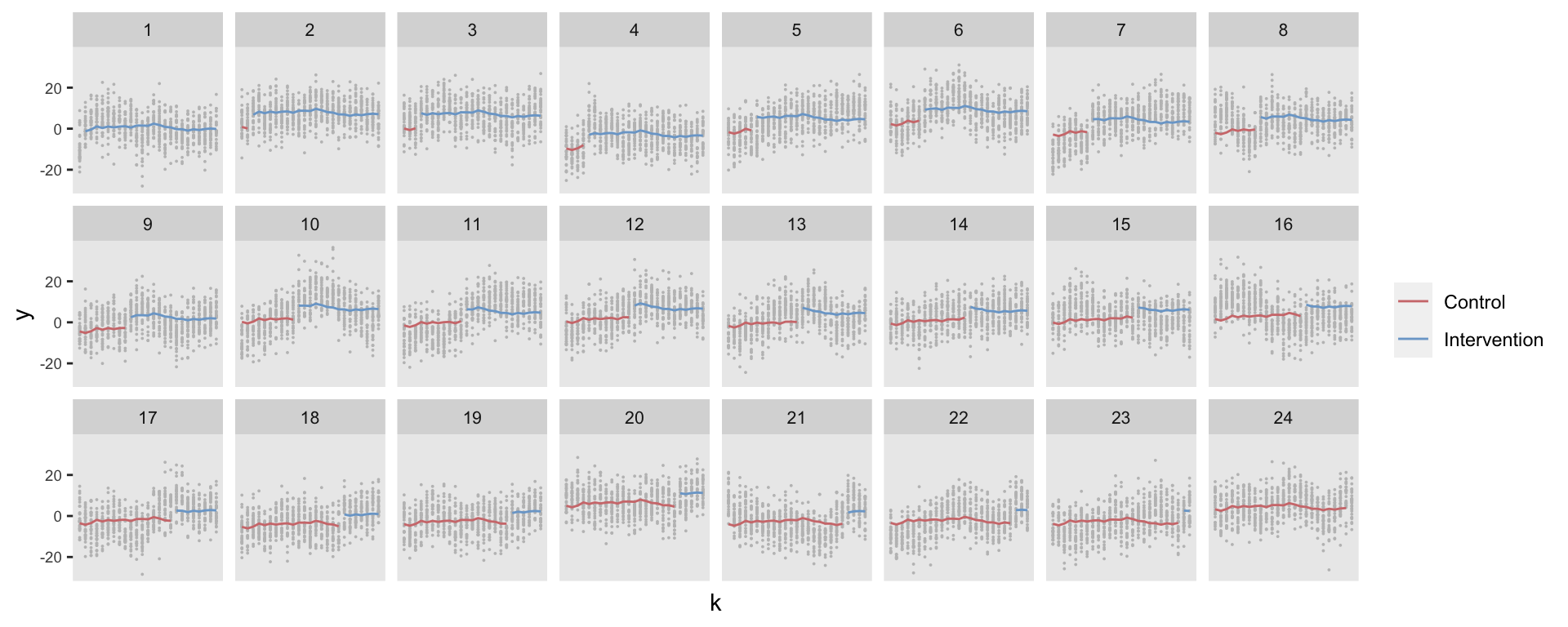
## factor(k)24 -1.31230 0.74417 -1.763The predicted values indicate that the model does not pick up the site-specific variation over time:
Although the estimate of the treatment effect from the single data set is 5.8 [95% CI: 5.5, 6.2], the treatment effect estimate from this model is actually unbiased (based on evaluating the results from the replications). However, RMSE = 0.97 (which is equivalent to the true standard error of the estimated treatment effect since there is no bias), but the average estimated standard error was only 0.18, and the coverage of the 95% CIs was only 29%. Indeed the estimated confidence interval from our single data set did not include the true value. Based on all of this, the model doesn’t seem all that promising, particularly with respect to measuring the uncertainty.
Mixed effects model with site-specific natural cubic spline
With the second model, also a mixed effects model, I’ve included a random cubic spline (based on four knots) instead of the random intercept:
dd[, normk := (k - min(k))/(max(k) - min(k))]
knots <- c(.2, .4, .6, .8)

fitlme_s <- lmer(y ~ A + ( ns(normk, knots = knots) - 1 | site ), data = dd)
summary(fitlme_s)
## Linear mixed model fit by REML ['lmerMod']
## Formula: y ~ A + (ns(normk, knots = knots) - 1 | site)
## Data: dd
##
## REML criterion at convergence: 120120.9
##
## Scaled residuals:
## Min 1Q Median 3Q Max
## -4.0707 -0.6768 0.0080 0.6671 4.1554
##
## Random effects:
## Groups Name Variance Std.Dev. Corr
## site ns(normk, knots = knots)1 30.97 5.565
## ns(normk, knots = knots)2 59.08 7.686 0.33
## ns(normk, knots = knots)3 28.10 5.301 0.12 -0.10
## ns(normk, knots = knots)4 75.10 8.666 0.16 0.55 -0.31
## ns(normk, knots = knots)5 28.28 5.318 0.49 0.14 0.58 -0.28
## Residual 45.25 6.727
## Number of obs: 18000, groups: site, 24
##
## Fixed effects:
## Estimate Std. Error t value
## (Intercept) -2.0677 0.1830 -11.30
## A 5.0023 0.3052 16.39
##
## Correlation of Fixed Effects:
## (Intr)
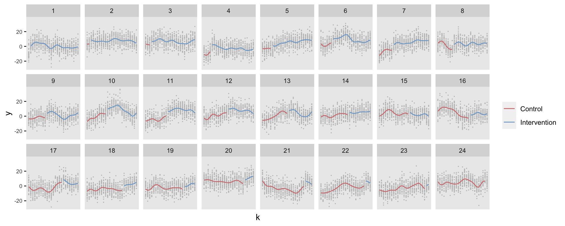
## A -0.088This time we can see that the model predictions better reflect the site-specific time trends:
This model also provides an unbiased estimate (in the case of the first data set, the estimate was spot on 5.0 [4.4, 5.6].) The RMSE was lower than the first model (0.78) and the average estimate of the standard error was slightly higher (0.31). The coverage was also higher, but still only 56%. There is still room for improvement.
GAM with site-specific smoother
This last model is a GAM (using the gam function from the mgcv package). A key parameter in the smoothing function s is the bs argument for the type of basis spline. I’ve used the option “fs” that allows for “random factor smooth interactions,” which is what we need here. In addition, the dimension of the basis (the argument k, not to be confused with the period k), was set by evaluating the selection criterion (GCV) as well investigating the RMSE and the average estimated standard errors. A value of k between 10 and 15 seems to be ideal, I’ve settled on \(k = 12\).
gamfit <- gam(y ~ A + s(k, site, bs = "fs", k = 12), data = dd)
summary(gamfit)
##
## Family: gaussian
## Link function: identity
##
## Formula:
## y ~ A + s(k, site, bs = "fs", k = 12)
##
## Parametric coefficients:
## Estimate Std. Error t value Pr(>|t|)
## (Intercept) -0.4595 0.7429 -0.619 0.536
## A 5.2864 0.4525 11.682 <2e-16 ***
## ---
## Signif. codes: 0 '***' 0.001 '**' 0.01 '*' 0.05 '.' 0.1 ' ' 1
##
## Approximate significance of smooth terms:
## edf Ref.df F p-value
## s(k,site) 261.7 287 32.8 <2e-16 ***
## ---
## Signif. codes: 0 '***' 0.001 '**' 0.01 '*' 0.05 '.' 0.1 ' ' 1
##
## R-sq.(adj) = 0.403 Deviance explained = 41.2%
## GCV = 41.693 Scale est. = 41.082 n = 18000The predicted value plot highlights that this model has estimated site-specific secular functions that are a little more wriggly than the cubic splines.
In spite of the less smooth curve, the GAM estimate is unbiased as well with a slightly lower RMSE (0.76) then the cubic spline model (0.78). Better yet, the estimated standard errors averaged 0.45, and the coverage is 76% (compared to 56% from the cubic spline model).
In general, at least in this simulation setting, the GAM seems to be an improvement over the random cubic spline model. However, this last model still underestimates the measure of uncertainty, suggesting there is more work to be done. Next, I will explore estimation of robust standard errors using bootstrap methods.
To be continued …