A new version of simstudy is available on CRAN. There are two major enhancements and several new features. In the “major” category, I would include (1) changes to survival data generation that accommodate hazard ratios that can change over time, as well as competing risks, and (2) the addition of functions to allow users to sample from existing data sets with replacement to generate “synthetic” data will real life distribution properties. Other less monumental, but important, changes were made: updates to functions genFormula and genMarkov, and two added utility functions, survGetParams and survParamPlot. (I did describe the survival data generation functions in two recent posts, here and here.)
Here are the highlights of the major enhancements:
Non-proportional hazards
If we want to simulate a scenario where survival time is a function of sex and the relative risk of death (comparing males to females) changes after 150 days, we cannot use the proportional hazards assumption that simstudy has typically assumed. Rather, we need to be able to specify different hazards at different time points. This is now implemented in simstudy by using the defSurv function and the transition argument.
In this case, the same outcome variable “death” is specified multiple times (currently the limit is actually two times) in defSurv, and the transition argument indicates the point at which the hazard ratio (HR) changes. In the example below, the log(HR) comparing males and females between day 0 and 150 is -1.4 (HR = 0.25), and after 150 days the hazards are more closely aligned, log(HR) = -0.3 (HR = 0.74). The data definitions determine the proportion of males in the sample and specify the time to death outcomes:
library(simstudy)
library(survival)
library(gtsummary)

def <- defData(varname = "male", formula = 0.5, dist = "binary")

defS <- defSurv(varname = "death", formula = "-14.6 - 1.4 * male",
  shape = 0.35, transition = 0)
defS <- defSurv(defS, varname = "death", formula = "-14.6 - 0.3 * male",
  shape = 0.35, transition = 150)
If we generate the data and take a look at the survival curves, it is possible to see a slight inflection point at 150 days where the HR shifts:
set.seed(10)

dd <- genData(600, def)
dd <- genSurv(dd, defS, digits = 2)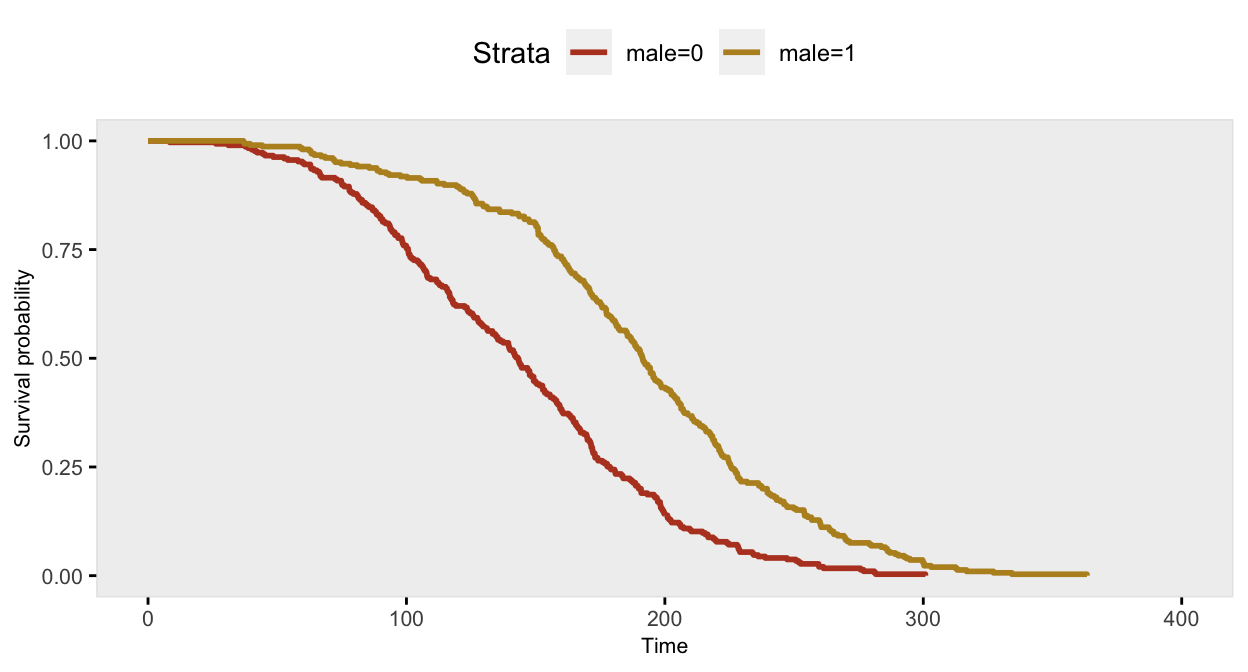
If we fit a standard Cox proportional hazard model and test the proportionality assumption, it is quite clear that the assumption is violated (as the p-value < 0.05):
coxfit <- coxph(formula = Surv(death) ~ male, data = dd)
cox.zph(coxfit)
## chisq df p
## male 12.5 1 0.00042
## GLOBAL 12.5 1 0.00042If we split the data at the proper inflection point of 150 days, and refit the model, we can recover the parameters (or at least get pretty close):
dd2 <- survSplit(Surv(death) ~ ., data= dd, cut=c(150),
                 episode= "tgroup", id="newid")

coxfit2 <- coxph(Surv(tstart, death, event) ~ male:strata(tgroup), data=dd2)

tbl_regression(coxfit2)| Characteristic | log(HR)1 | 95% CI1 | p-value |
|---|---|---|---|
| male * strata(tgroup) | |||
| male * tgroup=1 | -1.3 | -1.6, -1.0 | <0.001 |
| male * tgroup=2 | -0.51 | -0.72, -0.29 | <0.001 |
| 1 HR = Hazard Ratio, CI = Confidence Interval | |||
Competing risks
A new function addCompRisk generates a single time to event outcome from a collection of time to event outcomes, where the observed outcome is the earliest event time. This can be accomplished by specifying a timeName argument that will represent the observed time value. The event status is indicated in the field set by the eventName argument (which defaults to “event”). And if a variable name is indicated using the censorName argument, the censored events automatically have a value of 0.
To use addCompRisk, we first define and generate unique events - in this case event_1, event_2, and censor:
set.seed(1)

dS <- defSurv(varname = "event_1", formula = "-10", shape = 0.3)
dS <- defSurv(dS, "event_2", "-6.5", shape = 0.5)
dS <- defSurv(dS, "censor", "-7", shape = 0.55)

dtSurv <- genData(1001)
dtSurv <- genSurv(dtSurv, dS)

dtSurv
## id censor event_1 event_2
## 1: 1 55 15.0 9.7
## 2: 2 47 19.8 23.4
## 3: 3 34 8.0 33.1
## 4: 4 13 25.2 40.8
## 5: 5 61 28.6 18.9
## ---
## 997: 997 30 22.3 33.7
## 998: 998 53 22.3 20.5
## 999: 999 62 19.8 12.1
## 1000: 1000 55 11.1 22.1
## 1001: 1001 37 7.2 33.9Now we generate a competing risk outcome “obs_time” and an event indicator “delta”:
dtSurv <- addCompRisk(dtSurv, events = c("event_1", "event_2", "censor"),
  eventName = "delta", timeName = "obs_time", censorName = "censor")

dtSurv
## id obs_time delta type
## 1: 1 9.7 2 event_2
## 2: 2 19.8 1 event_1
## 3: 3 8.0 1 event_1
## 4: 4 13.0 0 censor
## 5: 5 18.9 2 event_2
## ---
## 997: 997 22.3 1 event_1
## 998: 998 20.5 2 event_2
## 999: 999 12.1 2 event_2
## 1000: 1000 11.1 1 event_1
## 1001: 1001 7.2 1 event_1Here’s a plot competing risk data using the cumulative incidence functions (rather than the survival curves):
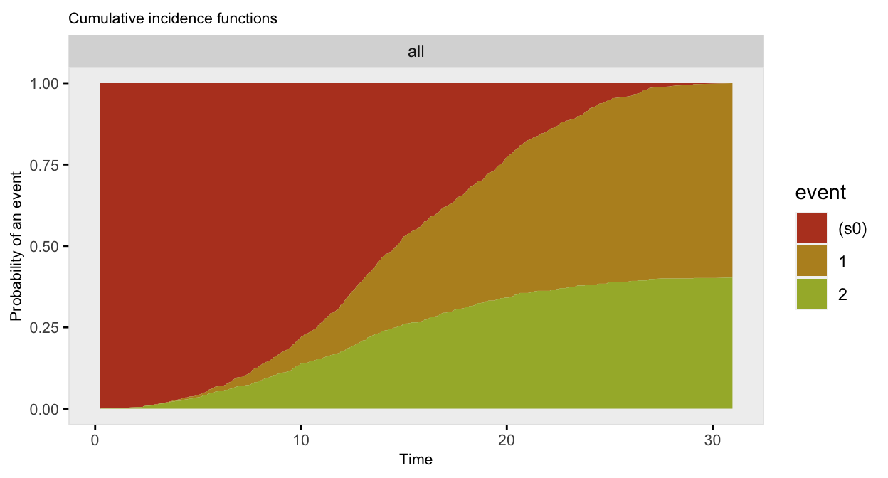
The data generation can be done in two (instead of three) steps by including the timeName and eventName arguments in the call to genSurv. By default, the competing events will be all the events defined in defSurv:
set.seed(1)

dtSurv <- genData(1001)
dtSurv <- genSurv(dtSurv, dS, timeName = "obs_time",
  eventName = "delta", censorName = "censor")

dtSurv
## id obs_time delta type
## 1: 1 9.7 2 event_2
## 2: 2 19.8 1 event_1
## 3: 3 8.0 1 event_1
## 4: 4 13.0 0 censor
## 5: 5 18.9 2 event_2
## ---
## 997: 997 22.3 1 event_1
## 998: 998 20.5 2 event_2
## 999: 999 12.1 2 event_2
## 1000: 1000 11.1 1 event_1
## 1001: 1001 7.2 1 event_1Synthetic data
Sometimes, it may be useful to generate data that will represent the distributions of an existing data set. Two new functions, genSynthetic and addSynthetic make it fairly easy to do this.
Let’s say we start with an existing data set \(A\) that has fields \(a\), \(b\), \(c\), and \(d\):
A## index a b c d
## 1: 1 2.74 8 0 11.1
## 2: 2 4.57 4 1 13.6
## 3: 3 2.63 4 0 8.0
## 4: 4 4.74 7 0 12.5
## 5: 5 1.90 4 0 7.2
## ---
## 996: 996 0.92 3 0 5.2
## 997: 997 2.89 4 0 8.5
## 998: 998 2.80 7 0 10.9
## 999: 999 2.47 6 0 8.1
## 1000: 1000 2.63 6 0 12.5We can create a synthetic data set by sampling records with replacement from data set \(A\):
S <- genSynthetic(dtFrom = A, n = 250, id = "index")
S
## index a b c d
## 1: 1 4.0 6 0 11.4
## 2: 2 3.2 4 1 9.5
## 3: 3 2.7 4 0 6.5
## 4: 4 1.7 4 0 6.2
## 5: 5 4.2 4 0 8.9
## ---
## 246: 246 1.1 5 0 6.5
## 247: 247 3.1 4 1 8.7
## 248: 248 3.3 2 0 1.2
## 249: 249 3.6 6 0 9.3
## 250: 250 3.1 3 0 6.2The distribution of variables in \(S\) matches their distribution in \(A\). Here are the univariate distributions for each variable in each data set:
summary(A[, 2:5])## a b c d
## Min. :0.0 Min. : 0.0 Min. :0.00 Min. : 0.1
## 1st Qu.:2.3 1st Qu.: 4.0 1st Qu.:0.00 1st Qu.: 6.9
## Median :3.0 Median : 5.0 Median :0.00 Median : 9.0
## Mean :3.0 Mean : 5.1 Mean :0.32 Mean : 9.1
## 3rd Qu.:3.8 3rd Qu.: 6.0 3rd Qu.:1.00 3rd Qu.:11.2
## Max. :6.0 Max. :13.0 Max. :1.00 Max. :18.1summary(S[, 2:5])## a b c d
## Min. :0.1 Min. : 0.0 Min. :0.00 Min. : 0.6
## 1st Qu.:2.3 1st Qu.: 3.0 1st Qu.:0.00 1st Qu.: 6.6
## Median :3.0 Median : 5.0 Median :0.00 Median : 8.6
## Mean :3.0 Mean : 4.7 Mean :0.33 Mean : 8.6
## 3rd Qu.:3.8 3rd Qu.: 6.0 3rd Qu.:1.00 3rd Qu.:10.5
## Max. :5.2 Max. :12.0 Max. :1.00 Max. :18.1And here are the covariance matrices for both:
cor(A[, cbind(a, b, c, d)])## a b c d
## a 1.0000 -0.0283 -0.0019 0.30
## b -0.0283 1.0000 0.0022 0.72
## c -0.0019 0.0022 1.0000 0.42
## d 0.3034 0.7212 0.4205 1.00cor(S[, cbind(a, b, c, d)])## a b c d
## a 1.000 0.033 -0.028 0.33
## b 0.033 1.000 0.052 0.76
## c -0.028 0.052 1.000 0.39
## d 0.335 0.764 0.388 1.00