As I mentioned last time, I am working on an update of simstudy that will make generating survival/time-to-event data a bit more flexible. I previously presented the functionality related to competing risks, and this time I’ll describe generating survival data that has time-dependent hazard ratios. (As I mentioned last time, if you want to try this at home, you will need the development version of simstudy that you can install using devtools::install_github(“kgoldfeld/simstudy”).)
Constant/proportional hazard ratio
In the current version of simstudy 0.4.0 on CRAN, the data generation process for survival/time-to-event outcomes can include covariates that effect the hazard rate (which is the risk/probability of having an event conditional on not having had experienced that event earlier). The ratio of hazards comparing different levels of a covariate are constant across all time points. For example, if we have a single binary covariate \(x\), the hazard \(\lambda(t)\) at time \(t\) is
\[\lambda(t|x) = \lambda_0(t) e ^ {\beta x}\]
where \(\lambda_0(t)\) is a baseline hazard when \(x=0\). The ratio of the hazards for \(x=1\) compared to \(x=0\) is
\[\frac{\lambda_0(t) e ^ {\beta}}{\lambda_0(t)} = e ^ \beta,\]
so the log of the hazard ratio is a constant \(\beta\), and the hazard ratio is always \(e^\beta\).
Here is a simulated example that assumes a constant log hazard ratio of \(-0.7\):
library(simstudy)
library(data.table)
library(survival)
def <- defData(varname = "x", formula = 0.4, dist = "binary")
defS <- defSurv(varname = "death", formula = "-14.6 - 0.7 * x", shape = 0.35)
defS <- defSurv(defS, varname = "censor", scale = exp(13), shape = 0.5)
set.seed(7361)
dd <- genData(500, def)
dd <- genSurv(dd, defS, digits = 2, timeName = "time", censorName = "censor")
dd## id x time event type
## 1: 1 0 164.98 1 death
## 2: 2 1 247.84 1 death
## 3: 3 0 28.54 1 death
## 4: 4 0 138.05 1 death
## 5: 5 0 228.53 1 death
## ---
## 496: 496 0 79.47 1 death
## 497: 497 1 5.41 0 censor
## 498: 498 1 211.54 1 death
## 499: 499 0 240.73 1 death
## 500: 500 1 256.66 1 deathThis is the Kaplan-Meier plot comparing survival curves for cases where \(x=0\) with cases where \(x=1\), which illustrates what a proportional hazard rate looks like:
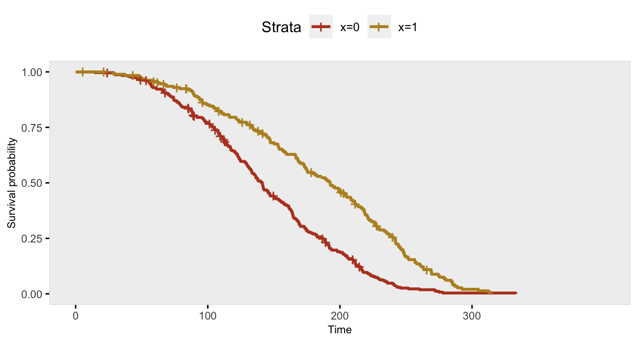
The Cox proportional hazards model recovers the correct log hazards rate:
coxfit <- coxph(formula = Surv(time, event) ~ x, data = dd)| Characteristic | log(HR)1 | 95% CI1 | p-value |
|---|---|---|---|
| x | -0.72 | -0.92, -0.52 | <0.001 |
| 1 HR = Hazard Ratio, CI = Confidence Interval | |||
Since we know that we used proportional hazards to generate the data, we can expect that a test evaluating the proportional hazards assumption using weighted residuals will confirm that the assumption is met. If the \(\text{p-value} < 0.05\), then we would conclude that the assumption of proportional hazards is not warranted. In this case \(p = 0.68\), so the model is apparently reasonable (which we already knew):
cox.zph(coxfit)## chisq df p
## x 0.17 1 0.68
## GLOBAL 0.17 1 0.68Non-constant/non-proportional hazard ratio
When generating data, we may not always want to be limited to a situation where the hazard ratio is constant over all time periods. To facilitate this, it is possible to specify two different data definitions for the same outcome, using the transition field to specify the point at which the second definition replaces the first. (While it would theoretically be possible to generate data for more than two periods, the process is more involved, and has not been implemented.)
In this next case, the risk of death when \(x=1\) is lower at all time points compared to when \(x=0\), but the relative risk (or hazard ratio) changes at 150 days:
def <- defData(varname = "x", formula = 0.4, dist="binary")
defS <- defSurv(varname = "death", formula = "-14.6 - 1.3 * x",
shape = 0.35, transition = 0)
defS <- defSurv(defS, varname = "death", formula = "-14.6 - 0.4 * x",
shape = 0.35, transition = 150)
defS <- defSurv(defS, varname = "censor", scale = exp(13), shape = 0.50)
dd <- genData(500, def)
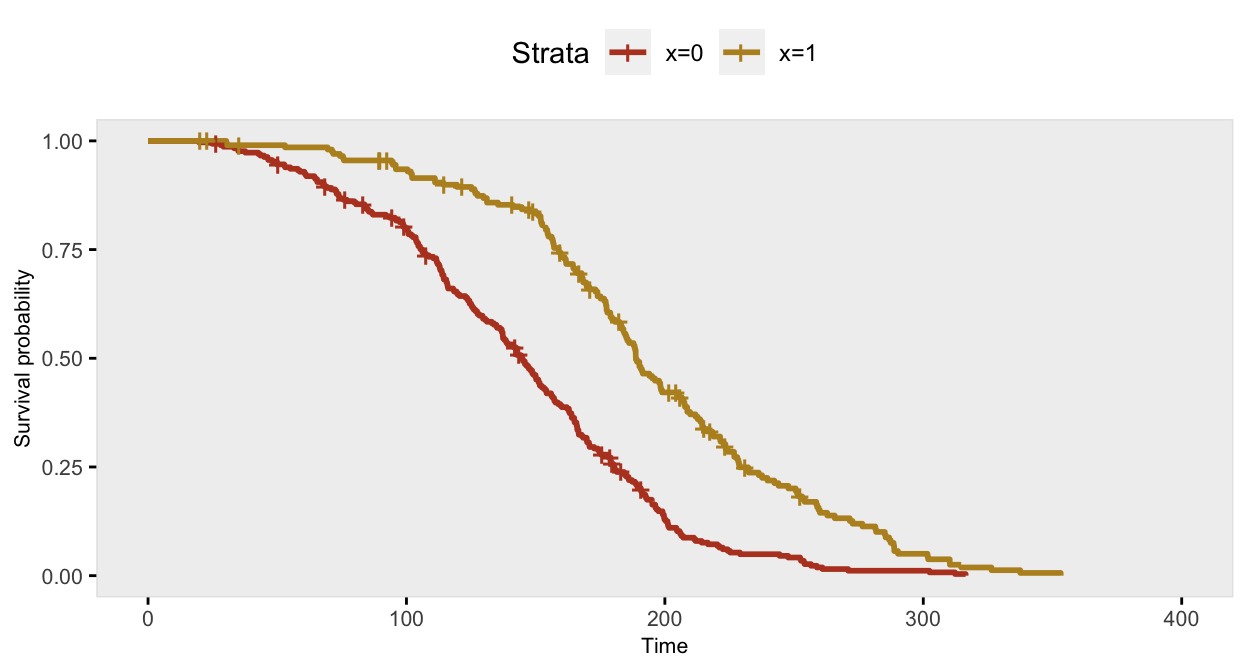
dd <- genSurv(dd, defS, digits = 2, timeName = "time", censorName = "censor")The survival curve for the sample with \(x=1\) has a slightly different shape under this data generation process compared to the previous example under a constant hazard ratio assumption; there is more separation early on (prior to day 150), and then the gap is closed at a quicker rate.
If we ignore the possibility that there might be a different relationship over time, the Cox proportional hazards model gives an estimate of the log hazard ratio quite close to -0.70:
coxfit <- survival::coxph(formula = Surv(time, event) ~ x, data = dd)| Characteristic | log(HR)1 | 95% CI1 | p-value |
|---|---|---|---|
| x | -0.84 | -1.0, -0.65 | <0.001 |
| 1 HR = Hazard Ratio, CI = Confidence Interval | |||
However, further inspection of the proportionality assumption should make us question the appropriateness of the model. Since \(p<0.05\), we would be wise to see if we can improve on the model.
cox.zph(coxfit)## chisq df p
## x 10.1 1 0.0015
## GLOBAL 10.1 1 0.0015We might be able to see from the plot where proportionality diverges, in which case we can split the data set into two parts at the identified time point. (In many cases, the transition point or points won’t be so obvious, in which case the investigation might be more involved.) By splitting the data at day 150, we get the desired estimates:
dd2 <- survSplit(Surv(time, event) ~ ., data= dd, cut=c(150),
                 episode= "tgroup", id="newid")

coxfit2 <- survival::coxph(Surv(tstart, time, event) ~ x:strata(tgroup), data=dd2)| Characteristic | log(HR)1 | 95% CI1 | p-value |
|---|---|---|---|
| x * strata(tgroup) | |||
| x * tgroup=1 | -1.5 | -1.8, -1.1 | <0.001 |
| x * tgroup=2 | -0.54 | -0.78, -0.29 | <0.001 |
| 1 HR = Hazard Ratio, CI = Confidence Interval | |||
And the diagnostic test of proportionality confirms the appropriateness of the model:
cox.zph(coxfit2)## chisq df p
## x:strata(tgroup) 1.38 2 0.5
## GLOBAL 1.38 2 0.5The actual data generation process implemented in simstudy is based on an algorithm described in this paper by Peter Austin.
Reference:
Austin, Peter C. “Generating survival times to simulate Cox proportional hazards models with time‐varying covariates.” Statistics in medicine 31, no. 29 (2012): 3946-3958.