An obvious downside to estimating Bayesian models is that it can take a considerable amount of time merely to fit a model. And if you need to estimate the same model repeatedly, that considerable amount becomes a prohibitive amount. In this post, which is part of a series (last one here) where I’ve been describing various aspects of the Bayesian analyses we plan to conduct for the COMPILE meta-analysis of convalescent plasma RCTs, I’ll present a somewhat elaborate model to illustrate how we have addressed these computing challenges to explore the properties of these models.
While concept of statistical power may not be part of the Bayesian analytic framework, there are many statisticians who would like to assess this property regardless of the modeling approach. These assessments require us to generate multiple data sets and estimate a model for each. In this case, we’ve found that each run through the MCMC-algorithm required to sample from the posterior probability of the Bayesian model can take anywhere from 7 to 15 minutes on our laptops or desktops. If we want to analyze 1,000 data sets using these methods, my laptop would need to run continuously for at least a week. And if we want to explore models under different assumptions about the data generating process or prior distributions - well, that would be impossible.
Fortunately, we have access to the High Performance Computing Core at NYU Langone Health (HPC), which enables us to analyze 1,000 data sets in about 90 minutes. Still pretty intensive, but clearly a huge improvement. This post describes how we adapted our simulation and modeling process to take advantage of the power and speed of the the HPC.
COMPILE Study design
There are numerous randomized control trials being conducted around the world to evaluate the efficacy of antibodies in convalescent blood plasma in improving outcomes for patients who have been hospitalized with COVID. Because each trial lacks adequate sample size to allow us to draw any definitive conclusions, we have undertaken a project to pool individual level data from these various studies into a single analysis. (I described the general approach and some conceptual issues here and here). The outcome is an 11-point categorical score developed by the WHO, with 0 indicating no COVID infection and 10 indicating death. As the intensity of support increases, the scores increase. For the primary outcome, the score will be based on patient status 14 days after randomization.
This study is complicated by the fact that each RCT is using one of three different control conditions: (1) usual care (unblinded), (2) non-convalescent plasma, and (3) saline solution. The model conceptualizes the three control conditions as three treatments to be compared against the reference condition of convalescent plasma. The overall treatment effect will represent a quantity centered around the three control effects.
Because we have access to individual-level data, we will be able to adjust for important baseline characteristics that might be associated with the prognosis at day 14; these are baseline WHO-score, age, sex, and symptom duration prior to randomization. The primary analysis will adjust for these factors, and secondary analyses will go further to investigate if any of these factors modify the treatment effect. In the example in this post, I will present the model based on a secondary analysis that considers only a single baseline factor symptom duration; we are allowing for the possibility that the treatment may be more or less effective depending on the symptom duration. (For example, patients who have been sicker longer may not respond to the treatment, while those who are treated earlier may.)
Model
Here is the model that I am using (as I mentioned, the planned COMPILE analysis will be adjusting for additional baseline characteristics):
\[ \text{logit} \left(P\left(Y_{kis} \ge y\right)\right) = \tau_{yk} + \beta_s + I_{ki} \left( \gamma_{kcs} + \delta_{kc} \right), \; \; y \in \{1, \dots L-1\} \text{ with } L \text{ response levels} \] And here are the assumptions for the prior distributions:
\[ \begin{aligned} \tau_{yk} &\sim t_{\text{student}} \left( \text{df=} 3, \mu=0, \sigma = 5 \right), \; \; \text{monotone within } \text{site } k \\ \beta_s &\sim \text{Normal} \left( \mu=0, \sigma = 5 \right), \qquad \; \;s \in \{1,\dots, S \} \text{ for symptom duration strata}, \beta_1 = 0 \\ \gamma_{kcs} &\sim \text{Normal}\left( \gamma_{cs}, 1 \right), \qquad \qquad \;\;\;\;\;\;c \in \{0, 1, 2\} \text{ for control conditions }, \gamma_{kc1} = 0 \text{ for all } k \\ \gamma_{cs} &\sim \text{Normal}\left( \Gamma_s, 0.25 \right), \qquad \qquad \; \; \gamma_{c1} = 0 \text{ for all } c \\ \Gamma_s &\sim t_{\text{student}} \left( 3, 0, 1 \right), \qquad \qquad \qquad \Gamma_{1} = 0 \\ \delta_{kc} &\sim \text{Normal}\left( \delta_c, \eta \right)\\ \delta_c &\sim \text{Normal}\left( -\Delta, 0.5 \right) \\ \eta &\sim t_{\text{student}}\left(3, 0, 0.25 \right) \\ -\Delta &\sim t_{\text{student}} \left( 3, 0, 2.5 \right) \end{aligned} \] There are \(K\) RCTs. The outcome for the \(i\)th patient from the \(k\)th trial on the \(L\)-point scale at day 14 is \(Y_{ki}=y\), \(y=0,\dots,L-1\) (although the COMPILE study will have \(L = 11\) levels, I will be using \(L=5\) to speed up estimation times a bit). \(I_{ki}\) indicates the treatment assignment for subject \(i\) in the \(k\)th RCT, \(I_{ki} = 0\) if patient \(i\) received CP and \(I_{ki} = 1\) if the patient was in any control arm. There are three control conditions \(C\): standard of care, \(C=0\); non-convalescent plasma, \(C=1\); saline/LR with coloring, \(C=2\); each RCT \(k\) is attached to a specific control condition. There are also \(S=3\) symptom duration strata: short duration, \(s=0\); moderate duration, \(s=1\); and long duration, \(s=2\). (COMPILE will use five symptom duration strata - again I am simplifying.)
\(\tau_{yk}\) corresponds to the \(k\)th RCT’s intercept associated with level \(y\); the \(\tau\)’s represent the cumulative log odds for patients with in symptom duration group \(s=0\) and receiving CP treatment. Within a particular RCT, all \(\tau_{yk}\)’s, satisfy the monotonicity requirements for the intercepts of the proportional odds model. \(\beta_s\), \(s \in {2, 3}\), is the main effect of symptom duration (\(\beta_1 = 0\), where \(s=1\) is the reference category). \(\gamma_{kcs}\) is the moderating effect of strata \(s\) in RCT \(k\); \(\gamma_{kc1} = 0\), since \(s=1\) is the reference category. \(\delta_{kc}\) is the RCT-specific control effect, where RCT \(k\) is using control condition \(c\).
Each \(\gamma_{kcs}\) is normally distributed around a control type/symptom duration mean \(\gamma_{cs}\). And each \(\gamma_{cs}\) is centered around a pooled mean \(\Gamma_s\). The \(\delta_{kc}\)’s are assumed to be normally distributed around a control-type specific effect \(\delta_c\), with variance \(\eta\) that will be estimated; the \(\delta_c\)’s are normally distributed around \(-\Delta\) (we take \(-\Delta\) as the mean of the distribution to which \(\delta_c\) belongs so that \(\exp(\Delta)\) will correspond to the cumulative log-odds ratio for CP relative to control, rather than for control relative to CP.). (For an earlier take on these types of models, see here.)
Go or No-go
The focus of a Bayesian analysis is the estimated posterior probability distribution of a parameter or parameters of interest, for example the log-odds ratio from a cumulative proportional odds model. At the end of an analysis, we have credibility intervals, means, medians, quantiles - all concepts associated a probability distribution.
A “Go/No-go” decision process like a hypothesis test is not necessarily baked into the Bayesian method. At some point, however, even if we are using a Bayesian model to inform our thinking, we might want to or have to make a decision. In this case, we might want recommend (or not) the use of CP for patients hospitalized with COVID-19. Rather than use a hypothesis test to reject or fail to reject a null hypothesis of no effect, we can use the posterior probability to create a decision rule. In fact, this is what we have done.
In the proposed design of COMPILE, the CP therapy will be deemed a success if both of these criteria are met:
\[ P \left( \exp\left(-\Delta\right) < 1 \right) = P \left( OR < 1 \right) > 95\%\]
\[P \left( OR < 0.80 \right) > 50\%\] The first statement ensures that the posterior probability of a good outcome is very high. If we want to be conservative, we can obviously increase the percentage threshold above \(95\%\). The second statement says that the there is decent probability that the treatment effect is clinically meaningful. Again, we can modify the target OR and/or the percentage threshold based on our desired outcome.
Goals of the simulation
Since there are no Type I or Type II errors in the Bayesian framework, the concept of power (which is the probability of rejecting the null hypothesis when it is indeed not true) does not logically flow from a Bayesian analysis. However, if we substitute our decision rules for a hypothesis test, we can estimate the probability (call it Bayesian power, though I imagine some Bayesians would object) that we will make a “Go” decision given a specified treatment effect. (To be truly Bayesian, we should impose some uncertainty on what that specific treatment effect is, and calculate a probability distribution of Bayesian power. But I am keeping things simpler here.)
Hopefully, I have provided sufficient motivation for the need to simulate data and fit multiple Bayesian models. So, let’s do that now.
The simulation
I am creating four functions that will form the backbone of this simulation process: s_define, s_generate, s_estimate, and s_extract. Repeated calls to each of these functions will provide us with the data that we need to get an estimate of Bayesian power under our (static) data generating assumptions.
Data definitions
The first definition table, defC1, sets up the RCTs. Each RCT has specific symptom duration interaction effect \(a\) and control treatment effect \(b\). To introduce a little variability in sample size, 1/3 of the studies will be larger (150 patients), and 2/3 will be smaller (75 patients).
The remaining tables, defC2, defS, and defC3, define patient-level data. defC2 adds the control group indicator (0 = CP, 1 = standard care, 2 = non-convalescent plasma, 3 = saline) and the symptom duration stratum. defS defines the interaction effect conditional on the stratum. defC3 defines the ordinal categorical outcome.
s_define <- function() {

  defC1 <- defDataAdd(varname = "a",formula = 0, variance = .005, dist = "normal")
  defC1 <- defDataAdd(defC1,varname = "b",formula = 0, variance= .01, dist = "normal")
  defC1 <- defDataAdd(defC1,varname = "size",formula = "75+75*large", dist = "nonrandom")

  defC2 <- defDataAdd(varname="C_rv", formula="C * control", dist = "nonrandom")
  defC2 <- defDataAdd(defC2, varname = "ss", formula = "1/3;1/3;1/3",
                      dist = "categorical")

  defS <- defCondition(
    condition = "ss==1",
    formula = 0,
    dist = "nonrandom")
  defS <- defCondition(defS,
    condition = "ss==2",
    formula = "(0.09 + a) * (C_rv==1) + (0.10 + a) * (C_rv==2) + (0.11 + a) * (C_rv==3)",
    dist = "nonrandom")
  defS <- defCondition(defS,
    condition = "ss==3",
    formula = "(0.19 + a) * (C_rv==1) + (0.20 + a) * (C_rv==2) + (0.21 + a) * (C_rv==3)",
    dist = "nonrandom")

  defC3 <- defDataAdd(
    varname = "z",
    formula = "0.1*(ss-1)+z_ss+(0.6+b)*(C_rv==1)+(0.7+b)*(C_rv==2)+(0.8+b)*(C_rv==3)",
    dist = "nonrandom")

  list(defC1 = defC1, defC2 = defC2, defS = defS, defC3 = defC3)

}
Data generation
The data generation process draws on the definition tables to create an instance of an RCT data base. This process includes a function genBaseProbs that I described previously.
s_generate <- function(deflist, nsites) {

  genBaseProbs <- function(n, base, similarity, digits = 2) {

    n_levels <- length(base)

    x <- gtools::rdirichlet(n, similarity * base)

    x <- round(floor(x*1e8)/1e8, digits)
    xpart <- x[, 1:(n_levels-1)]
    partsum <- apply(xpart, 1, sum)
    x[, n_levels] <- 1 - partsum

    return(x)
  }

  basestudy <- genBaseProbs(n = nsites,
                            base =  c(.10, .35, .25, .20, .10),
                            similarity = 100)

  dstudy <- genData(nsites, id = "study")
  dstudy <- trtAssign(dstudy, nTrt = 3, grpName = "C")
  dstudy <- trtAssign(dstudy, nTrt = 2, strata = "C", grpName = "large", ratio = c(2,1))
  dstudy <- addColumns(deflist[['defC1']], dstudy)

  dind <- genCluster(dstudy, "study", numIndsVar = "size", "id")
  dind <- trtAssign(dind, strata="study", grpName = "control")
  dind <- addColumns(deflist[['defC2']], dind)
  dind <- addCondition(deflist[["defS"]], dind, newvar = "z_ss")
  dind <- addColumns(deflist[['defC3']], dind)

  dl <- lapply(1:nsites, function(i) {
    b <- basestudy[i,]
    dx <- dind[study == i]
    genOrdCat(dx, adjVar = "z", b, catVar = "ordY")
  })

  rbindlist(dl)[]
}
Model estimation
The estimation involves creating a data set for Stan and sampling from the Bayesian model. The Stan model is included in the addendum.
s_estimate <- function(dd, s_model) {

  N <- nrow(dd)                               ## number of observations
  L <- dd[, length(unique(ordY))]             ## number of levels of outcome
  K <- dd[, length(unique(study))]            ## number of studies
  y <- as.numeric(dd$ordY)                    ## individual outcome
  kk <- dd$study                              ## study for individual
  ctrl <- dd$control                          ## treatment arm for individual
  cc <- dd[, .N, keyby = .(study, C)]$C       ## specific control arm for study
  ss <- dd$ss
  x <- model.matrix(ordY ~ factor(ss), data = dd)[, -1]

  studydata <- list(N=N, L= L, K=K, y=y, kk=kk, ctrl=ctrl, cc=cc, ss=ss, x=x)

  fit <-  sampling(s_model, data=studydata, iter = 4000, warmup = 500,
                   cores = 4L, chains = 4, control = list(adapt_delta = 0.8))
  fit
}
Estimate extraction
The last step is the extraction of summary data from the posterior probability distributions. I am collecting quantiles of the key parameters, including \(\Delta\) and \(OR = \exp(-\Delta)\). For the Bayesian power analysis, I am estimating the probability of falling below the two thresholds for each data set. And finally, I want to get a sense of the quality of each estimation process by recovering the number of divergent chains that resulted from the MCMC algorithm (more on that here).
s_extract <- function(iternum, mcmc_res) {

  posterior <- as.array(mcmc_res)

  x <- summary(
    mcmc_res,
    pars = c("Delta", "delta", "Gamma", "beta", "alpha", "OR"),
    probs = c(0.025, 0.5, 0.975)
  )

  dpars <- data.table(iternum = iternum, par = rownames(x$summary), x$summary)

  p.eff <- mean(rstan::extract(mcmc_res, pars = "OR")[[1]] < 1)
  p.clinic <- mean(rstan::extract(mcmc_res, pars = "OR")[[1]] < 0.8)
  dp <- data.table(iternum = iternum, p.eff = p.eff, p.clinic = p.clinic)

  sparams <- get_sampler_params(mcmc_res, inc_warmup=FALSE)
  n_divergent <- sum(sapply(sparams, function(x) sum(x[, 'divergent__'])))
  ddiv <- data.table(iternum, n_divergent)

  list(ddiv = ddiv, dpars = dpars, dp = dp)
}
Replication
Now we want to put all these pieces together and repeatedly execute those four functions and save the results from each. I’ve described using lapply to calculate power in a much more traditional setting. We’re going to take the same approach here, except on steroids, replacing lapply not with mclapply, the parallel version, but with Slurm_lapply, which is a function in the slurmR package.
Slurm (Simple Linux Utility for Resource Management) is a HPC cluster job scheduler. slurmR is a wrapper that mimics many of the R parallel package functions, but in a Slurm environment. The strategy here is to define a meta-function (iteration) that itself calls the four functions already described, and then call that function repeatedly. Slurm_lapply does that, and rather than allocating the iterations to different cores on a computer like mclapply does, it allocates the iterations to different nodes on the HPC, using what is technically called a job array. Each node is essentially its own computer. In addition to that, each node has multiple cores, so we can run the different MCMC chains in parallel within a node; we have parallel processes within a parallel process. I have access to 100 nodes at any one time, though I find I don’t get much performance improvement if I go over 90, so that is what I do here. Within each node, I am using 4 cores. I am running 1,980 iterations, so that is 22 iterations per node. As I mentioned earlier, all of this runs in about an hour and a half.
The following code includes the “meta-function” iteration, the compilation of the Stan model (which only needs to be done once, thankfully), the Slurm_lapply call, and the Slurm batch code that I need to execute to get the whole process started on the HPC, which is called Big Purple here at NYU. (All of the R code goes into a single .R file, the batch code is in a .slurm file, and the Stan code is in its own .stan file.)
iteration <- function(iternum, s_model, nsites) {

    s_defs <- s_define()
    s_dd <- s_generate(s_defs, nsites = nsites)
    s_est <- s_estimate(s_dd, s_model)
    s_res <- s_extract(iternum, s_est)

    return(s_res)

}
library(simstudy)
library(rstan)
library(data.table)
library(slurmR)
rt <- stanc("/.../r/freq_bayes.stan")
sm <- stan_model(stanc_ret = rt, verbose=FALSE)
job <- Slurm_lapply(
X = 1:1980,
iteration,
s_model = sm,
nsites = 9,
njobs = 90,
mc.cores = 4,
tmp_path = "/.../scratch",
overwrite = TRUE,
job_name = "i_fb",
sbatch_opt = list(time = "03:00:00", partition = "cpu_short"),
export = c("s_define", "s_generate", "s_estimate", "s_extract"),
plan = "wait")
job
res <- Slurm_collect(job)
diverge <- rbindlist(lapply(res, function(l) l[["ddiv"]]))
ests <- rbindlist(lapply(res, function(l) l[["dpars"]]))
probs <- rbindlist(lapply(res, function(l) l[["dp"]]))
save(diverge, ests, probs, file = "/.../data/freq_bayes.rda")#!/bin/bash
#SBATCH --job-name=fb_parent
#SBATCH --mail-type=END,FAIL # send email if the job end or fail
#SBATCH --mail-user=keith.goldfeld@nyulangone.org
#SBATCH --partition=cpu_short
#SBATCH --time=3:00:00 # Time limit hrs:min:sec
#SBATCH --output=fb.out # Standard output and error log
module load r/3.6.3
cd /.../r
Rscript --vanilla fb.RResults
Each of the three extracted data tables are combined across simulations and the results are saved to an .rda file, which can be loaded locally in R and summarized. In this case, we are particularly interested in the Bayesian power estimate, which is the proportion of data sets that would results in a “go” decision (a recommendation to strongly consider using the intervention).
However, before we consider that, we should first get a rough idea about how many replications had divergence issues, which we extracted into the diverge data table. For each replication, we used four chains of length 3,500 each (after the 500 warm-up samples), accounting for a total of 14,000 chains. Here are the proportion of replications with at least one divergent chain:
load("DataBayesCOMPILE/freq_bayes.rda")
diverge[, mean(n_divergent > 0)]
## [1] 0.102While 10% of replications with at least 1 divergent chain might seem a little high, we can get a little more comfort from the fact that it appears that almost all replications had fewer than 35 (0.25%) divergent chains:
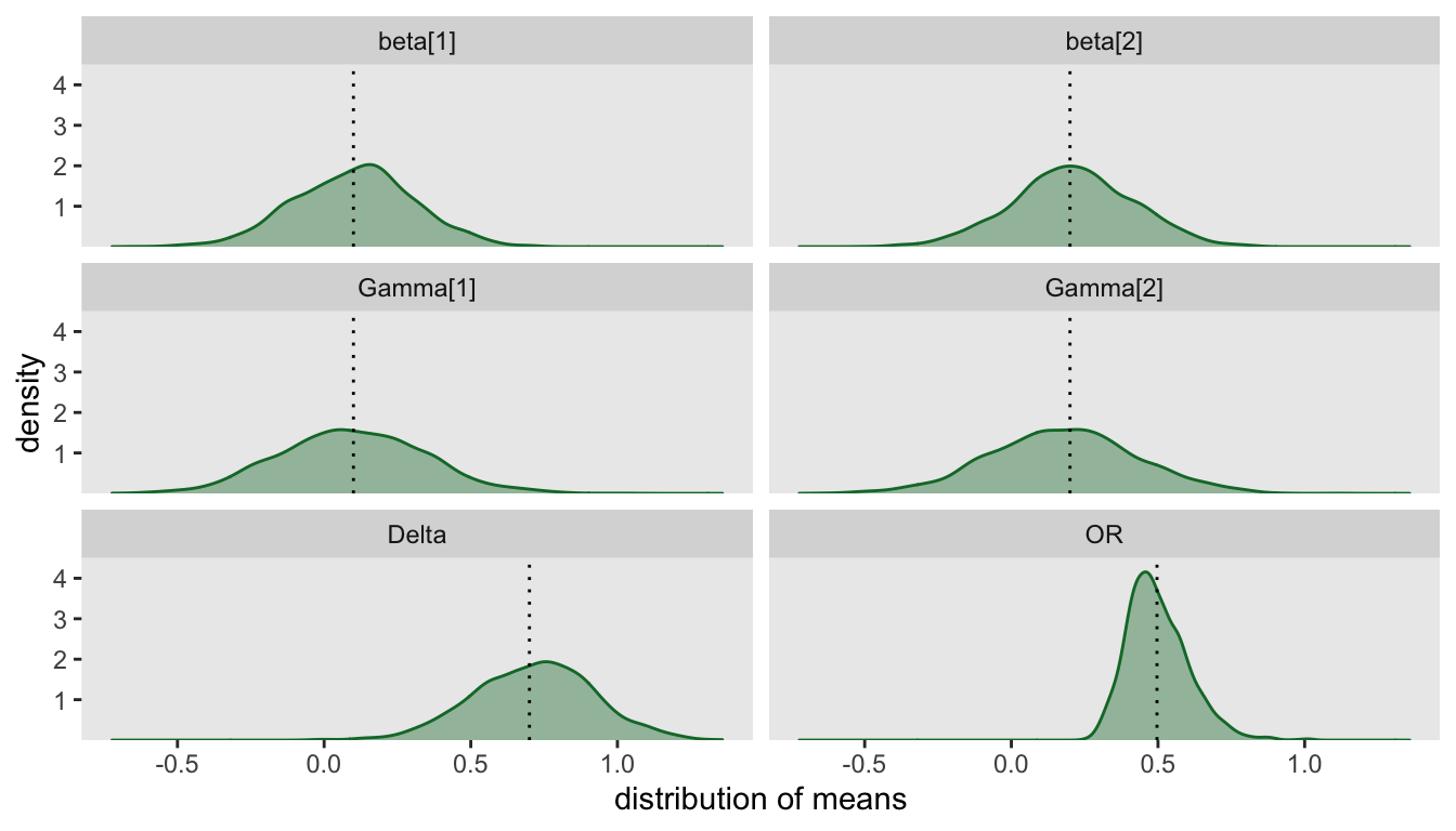
diverge[, mean(n_divergent < 35)]## [1] 0.985To get a general sense of how well our model is working, we can plot the distribution of posterior medians. In particular, this will allow us to assess how well the model is recovering the values used in the data generating process. In this case, I am excluding the 29 replications with 35 or more divergent chains:
Finally, we are ready to report the estimated Bayesian power (again, using the replications with limited number of divergent chains) and show the distribution of probabilities.
probs_d <- merge(probs, diverge, by = "iternum")[n_divergent < 35]
probs_d[, mean(p.eff > 0.95 & p.clinic > 0.50)]
## [1] 0.726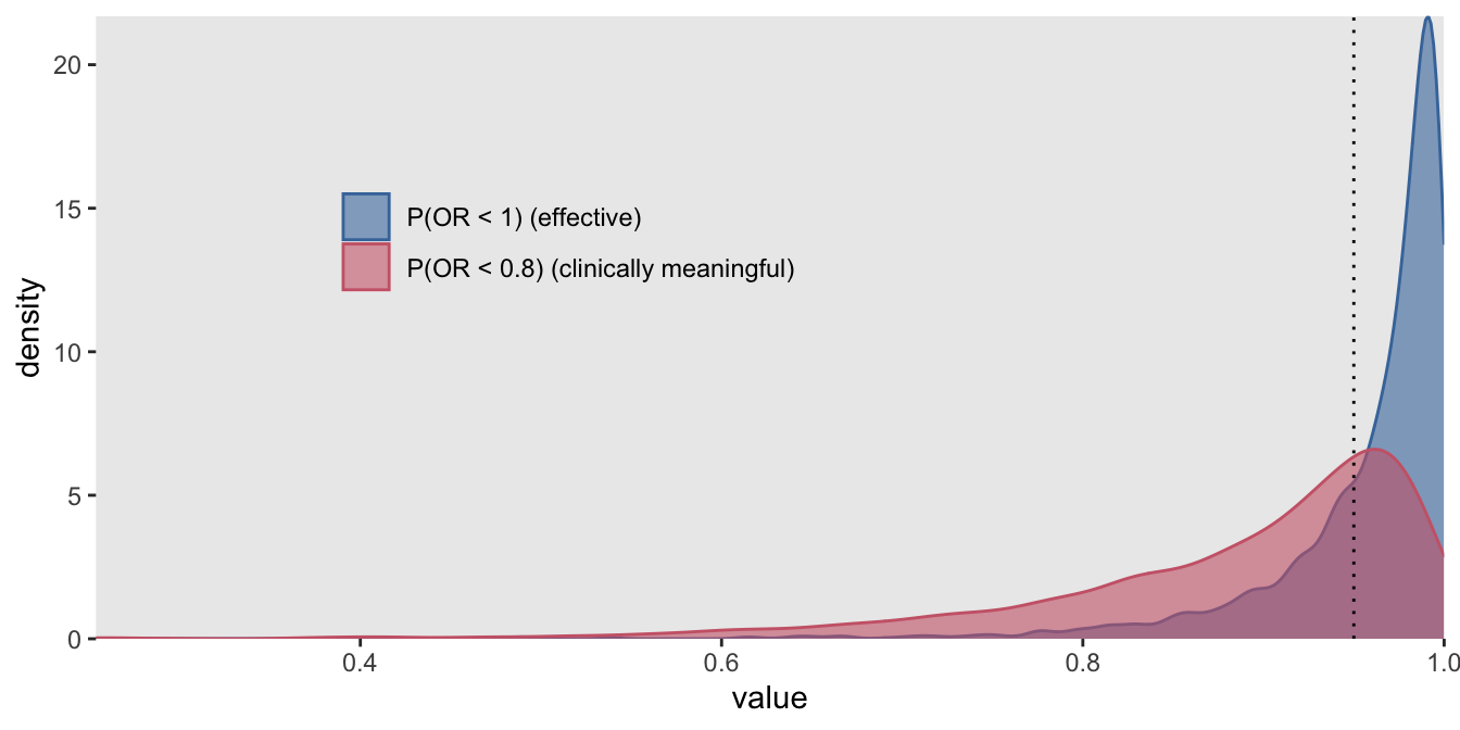
So, given an actual effect \(OR=\exp(-0.70) = 0.50\), we would conclude with a decision to go ahead with the therapy with 73% probability. However, a single estimate of power based on one effect size is a bit incomplete; it would be preferable to assess power under numerous scenarios of effect sizes and perhaps prior distribution assumptions to get a more complete picture. And if you have access to a HPC, this may actually be something you can do in a realistic period of time.
Addendum
The stan model that implements the model described at the outset actually looks a little different than that model in two key ways. First, there is a parameter \(\alpha\) that appears in the outcome model, which represents an overall intercept across all studies. Ideally, we wouldn’t need to include this parameter since we want to fix it at zero, but the model behaves very poorly without it. We do include it, but with a highly restrictive prior that will constrain it to be very close to zero. The second difference is that standard normal priors appear in the model - this is to alleviate issues related to divergent chains, which I described in a previous post.
data {
    int<lower=0> N;                // number of observations
    int<lower=2> L;                // number of WHO categories
    int<lower=1> K;                // number of studies
    int<lower=1,upper=L> y[N];     // vector of categorical outcomes
    int<lower=1,upper=K> kk[N];    // site for individual
    int<lower=0,upper=1> ctrl[N];  // treatment or control
    int<lower=1,upper=3> cc[K];    // specific control for site
    int<lower=1,upper=3> ss[N];    // strata
    row_vector[2] x[N];            // strata indicators  N x 2 matrix
  }

parameters {

  real Delta;               // overall control effect
  vector[2] Gamma;          // overall strata effect
  real alpha;               // overall intercept for treatment
  ordered[L-1] tau[K];      // cut-points for cumulative odds model (K X [L-1] matrix)

  real<lower=0>  eta_0;     // sd of delta_k (around delta)

  // non-central parameterization

  vector[K] z_ran_rx;      // site-specific effect
  vector[2] z_phi[K];      // K X 2 matrix
  vector[3] z_delta;
  vector[2] z_beta;
  vector[2] z_gamma[3];    // 3 X 2 matrix
}

transformed parameters{

  vector[3] delta;          // control-specific effect
  vector[K] delta_k;        // site specific treatment effect
  vector[2] gamma[3];       // control-specific duration strata effect (3 X 2 matrix)
  vector[2] beta;           // covariate estimates of ss
  vector[2] gamma_k[K];     // site-specific duration strata effect (K X 2 matrix)
  vector[N] yhat;


  delta = 0.5 * z_delta + Delta; // was 0.1
  beta = 5 * z_beta;

  for (c in 1:3)
    gamma[c] = 0.25 * z_gamma[c] + Gamma;

  for (k in 1:K){
    delta_k[k] = eta_0 * z_ran_rx[k] + delta[cc[k]];
  }

  for (k in 1:K)
    gamma_k[k] = 1 * z_phi[k] + gamma[cc[k]];

  for (i in 1:N)
    yhat[i] = alpha + x[i] * beta + ctrl[i] * (delta_k[kk[i]] + x[i]*gamma_k[kk[i]]);
}

model {

  // priors

  z_ran_rx ~ std_normal();
  z_delta ~ std_normal();
  z_beta ~ std_normal();

  alpha ~ normal(0, 0.25);
  eta_0 ~ student_t(3, 0, 0.25);

  Delta ~ student_t(3, 0, 2.5);
  Gamma ~ student_t(3, 0, 1);

  for (c in 1:3)
      z_gamma[c] ~ std_normal();

  for (k in 1:K)
      z_phi[k] ~ std_normal();

  for (k in 1:K)
      tau[k] ~ student_t(3, 0, 5);

  // outcome model

  for (i in 1:N)
    y[i] ~ ordered_logistic(yhat[i], tau[kk[i]]);
}

generated quantities {

  real OR;
  OR = exp(-Delta);

}