Over the past couple of months, I’ve been describing various aspects of the simulations that we’ve been doing to get ready for a meta-analysis of convalescent plasma treatment for hospitalized patients with COVID-19, most recently here. As I continue to do that, I want to provide motivation and code for a small but important part of the data generating process, which involves creating probabilities for ordinal categorical outcomes using a Dirichlet distribution.
Motivation
The outcome for the analysis that we will be conducting is the WHO 11-point ordinal scale for clinical improvement at 14 days, which ranges from 0 (uninfected and out of the hospital) to 10 (dead), with various stages of severity in between. We plan to use a Bayesian proportional odds model to assess the effectiveness of the therapy. Since this is a meta-analysis, we will be including these data from a collection of studies being conducted around the world.
Typically, in a proportional odds model one has to make an assumption about proportionality. In this case, while we are willing to make that assumption within specific studies, we are not willing to make that assumption across the various studies. This means we need to generate a separate set of intercepts for each study that we simulate.
In the proportional odds model, we are modeling the log-cumulative odds at a particular level. The simplest model with a single exposure/treatment covariate for a specific study or cluster is
where ranges from 1 to 10, all the levels of the WHO score excluding the lowest level . is the treatment indicator, and is for patients who receive the treatment. is the intercept for each study/cluster . is interpreted as the log-odds ratio comparing the odds of the treated with the non-treated within each study. The proportionality assumption kicks in here when we note that is constant for all levels of . In addition, in this particular model, we are assuming that the log-odds ratio is constant across studies (not something we will assume in a more complete model). We make no assumptions about how the study intercepts relate to each other.
To make clear what it would mean to make a stronger assumption about the odds across studies consider this model:
where the intercepts for each study are related, since they are defined as , and share in common. If we compare the log-odds of the treated in one study with the log-odds of treated in another study (so in both cases), the log-odds ratio is . The ratio is independent of , which implies a strong proportional odds assumption across studies. In contrast, the same comparison across studies based on the first model is , which is not necessarily constant across different levels of .
This is a long way of explaining why we need to generate different sets of intercepts for each study. In short, we would like to make the more relaxed assumption that odds are not proportional across studies or clusters.
The Dirichlet distribution
In order to generate ordinal categorical data I use the genOrdCat function in the simstudy package. This function requires a set of baseline probabilities that sum to one; these probabilities map onto level-specific intercepts. There will be a distinct set of baseline probabilities for each study and I will create a data set for each study. The challenge is to be able to generate unique baseline probabilities as if I were sampling from a population of studies.
If I want to generate a single probability (i.e. a number between and ), a good solution is to draw a value from a beta distribution, which has two shape parameters and .
Here is a single draw from :
set.seed(872837)

rbeta(1, shape1 = 3, shape2 = 3)
## [1] 0.568The mean of the beta distribution is and the variance is . We can reduce the variance and maintain the same mean by increasing and by a constant factor (see addendum for a pretty picture):
library(data.table)

d1 <- data.table(s = 1, value = rbeta(1000, shape1 = 1, shape2 = 2))
d2 <- data.table(s = 2, value = rbeta(1000, shape1 = 5, shape2 = 10))
d3 <- data.table(s = 3, value = rbeta(1000, shape1 = 100, shape2 = 200))

dd <- rbind(d1, d2, d3)
dd[, .(mean(value), sd(value)), keyby = s]
## s V1 V2
## 1: 1 0.338 0.2307
## 2: 2 0.336 0.1195
## 3: 3 0.333 0.0283The Dirichlet distribution is a multivariate version of the beta distribution where values between and are generated, with the caveat that they sum to . Instead of and , the Dirichlet is parameterized by a vector of length
where there are levels of the ordinal outcome. A draw from this distribution returns a vector where and
A draw from a Dirichlet distribution with is actually equivalent to a draw from a beta distribution where . Before, I generated data from a , and now here is a draw from using rdirichlet from the gtools package:
library(gtools)

dir <- rdirichlet(1000, alpha = c(1,2))
head(dir)
## [,1] [,2]
## [1,] 0.3606 0.639
## [2,] 0.4675 0.533
## [3,] 0.2640 0.736
## [4,] 0.0711 0.929
## [5,] 0.5643 0.436
## [6,] 0.0188 0.981The first column has the same distribution as the distribution from before; the mean and standard deviation are close to the values estimated above:
c(mean(dir[,1]), sd(dir[,1]))## [1] 0.332 0.236To ramp things up a bit, say we have , and the target mean values for each level are , one way to specify this is:
dir_1 <- rdirichlet(1000, alpha = c(1, 2, 3, 2, 1))
head(dir_1)
## [,1] [,2] [,3] [,4] [,5]
## [1,] 0.1710 0.6637 0.0676 0.0633 0.0343
## [2,] 0.1130 0.1150 0.2803 0.4229 0.0689
## [3,] 0.1434 0.0678 0.3316 0.1721 0.2851
## [4,] 0.0250 0.1707 0.3841 0.2490 0.1712
## [5,] 0.0633 0.3465 0.4056 0.0853 0.0993
## [6,] 0.1291 0.1510 0.3993 0.2612 0.0593Here are the observed means for each , pretty close to the target:
apply(dir_1, 2, mean)## [1] 0.111 0.221 0.328 0.229 0.112Of course, we could generate data with a similar target by multiplying by a constant . In this case, we use and see that the average values for each are also close to the target:
dir_2 <- rdirichlet(1000, alpha = c(10, 20, 30, 20, 10))
apply(dir_2, 2, mean)
## [1] 0.113 0.222 0.334 0.220 0.111There is a key difference between specifying and . Just as in the beta distribution, as grows larger, the variation within each decreases. This will be useful when generating the study specific probabilities if we want explore different levels of variation.
Here’s the standard deviations from the two data sets just generated:
apply(dir_1, 2, sd)## [1] 0.102 0.131 0.144 0.134 0.098apply(dir_2, 2, sd)## [1] 0.0333 0.0425 0.0508 0.0421 0.0333Generating the baseline probabilities
A simple function that includes two key arguments - the base probabilities (which are really ) and a similarity index (which is really just the constant ) - implements these ideas to generate study-specific probabilities for each outcome level. As the similarity index increases, the variation across studies or sites decreases. The function includes an additional adjustment to ensure that the row totals sum exactly to and not to some value infinitesimally greater than as a result of rounding. Such a rounding error could cause problems for the function genOrdCat.
genBaseProbs <- function(n, base, similarity, digits = 8) {

  n_levels <- length(base)
  x <- rdirichlet(n, similarity * base)

  #--- ensure that each vector of probabilities sums exactly to 1

  x <- round(floor(x*1e8)/1e8, digits)   # round the generated probabilities
  xpart <- x[, 1:(n_levels-1)]           # delete the base prob of the final level
  partsum <- apply(xpart, 1, sum)        # add the values of levels 1 to K-1
  x[, n_levels] <- 1 - partsum           # the base prob of the level K = 1 - sum(1:[K-1])

  return(x)
}
In this first example, I am generating 11 values (representing base probabilities) for each of 9 studies using a relatively low similarity index, showing you the first six studies:
basestudy <- genBaseProbs(
  n = 9,
  base =  c(0.05, 0.06, 0.07, 0.11, 0.12, 0.20, 0.12, 0.09, 0.08, 0.05, 0.05),
  similarity = 15,
)

round(head(basestudy), 3)
## [,1] [,2] [,3] [,4] [,5] [,6] [,7] [,8] [,9] [,10] [,11]
## [1,] 0.094 0.022 0.121 0.100 0.061 0.102 0.053 0.309 0.059 0.078 0.000
## [2,] 0.025 0.079 0.043 0.197 0.083 0.044 0.099 0.148 0.025 0.150 0.107
## [3,] 0.007 0.042 0.084 0.066 0.049 0.145 0.191 0.323 0.078 0.012 0.003
## [4,] 0.061 0.021 0.063 0.104 0.092 0.292 0.112 0.110 0.113 0.026 0.008
## [5,] 0.067 0.023 0.021 0.042 0.063 0.473 0.108 0.127 0.016 0.013 0.046
## [6,] 0.001 0.018 0.054 0.225 0.150 0.301 0.043 0.081 0.100 0.008 0.020A great way to see the variability is a cumulative probability plot for each individual study. With a relatively low similarity index, you can generate quite a bit of variability across the studies. In order to create the plot, I need to first calculate the cumulative probabilities:
library(ggplot2)
library(viridis)

cumprobs <- data.table(t(apply(basestudy, 1, cumsum)))
n_levels <- ncol(cumprobs)
cumprobs[, id := .I]

dm <- melt(cumprobs, id.vars = "id", variable.factor = TRUE)
dm[, level := factor(variable, labels = c(0:10))]

ggplot(data  = dm, aes(x=level, y = value)) +
  geom_line(aes(group = id, color = id)) +
  scale_color_viridis( option = "D") +
  theme(panel.grid.minor = element_blank(),
        panel.grid.major.y = element_blank(),
        legend.position = "none")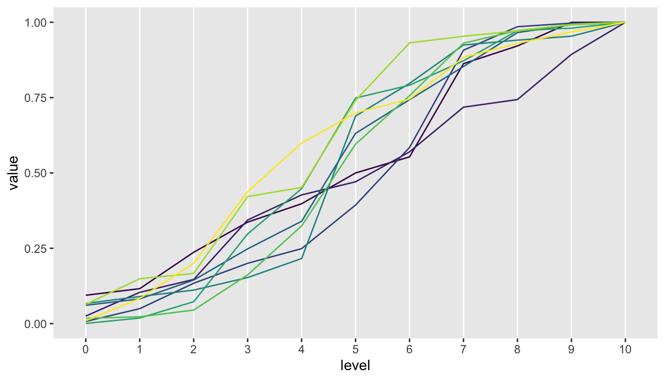
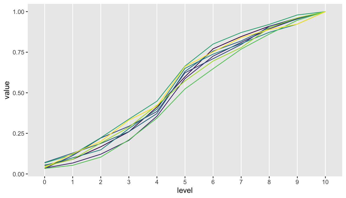
Here is a plot of data generated using a similarity index of 150. Variation is reduced pretty dramatically:
Using base probabilities to generate ordinal data
Now that we have these base probabilities, the last step is to use them to generate ordinal outcomes. I am generating the simplest of data sets: 9 “studies” each with 500 subjects, without any covariates or even treatment assignment. Since the genOrdCat requires an adjustment variable, I am adjusting everyone by 0. (This is something I need to fix - there should be no such requirement.)
library(simstudy)

d_study <- genData(9, id = "study")
d_ind <- genCluster(d_study, "study", numIndsVar = 500, "id")
d_ind[, z := 0]

d_ind
## study id z
## 1: 1 1 0
## 2: 1 2 0
## 3: 1 3 0
## 4: 1 4 0
## 5: 1 5 0
## ---
## 4496: 9 4496 0
## 4497: 9 4497 0
## 4498: 9 4498 0
## 4499: 9 4499 0
## 4500: 9 4500 0To generate the ordinal categorical outcome, we have to treat each study separately since they have unique baseline probabilities. This can be accomplished using lapply in the following way:
basestudy <- genBaseProbs(
  n = 9,
  base =  c(0.05, 0.06, 0.07, 0.11, 0.12, 0.20, 0.12, 0.09, 0.08, 0.05, 0.05),
  similarity = 50
)

list_ind  <- lapply(
  X = 1:9,
  function(i) {
    b <- basestudy[i,]
    d_x <- d_ind[study == i]
    genOrdCat(d_x, adjVar = "z", b, catVar = "ordY")
  }
)
The output list_ind is a list of data tables, one for each study. For example, here is the 5th data table in the list:
list_ind[[5]]## study id z ordY
## 1: 5 2001 0 7
## 2: 5 2002 0 9
## 3: 5 2003 0 5
## 4: 5 2004 0 9
## 5: 5 2005 0 9
## ---
## 496: 5 2496 0 9
## 497: 5 2497 0 4
## 498: 5 2498 0 7
## 499: 5 2499 0 5
## 500: 5 2500 0 11And here is a table of proportions for each study that we can compare with the base probabilities:
t(sapply(list_ind, function(x) x[, prop.table(table(ordY))]))## 1 2 3 4 5 6 7 8 9 10 11
## [1,] 0.106 0.048 0.086 0.158 0.058 0.162 0.092 0.156 0.084 0.028 0.022
## [2,] 0.080 0.024 0.092 0.134 0.040 0.314 0.058 0.110 0.028 0.110 0.010
## [3,] 0.078 0.050 0.028 0.054 0.148 0.172 0.162 0.134 0.058 0.082 0.034
## [4,] 0.010 0.056 0.116 0.160 0.054 0.184 0.102 0.084 0.156 0.056 0.022
## [5,] 0.010 0.026 0.036 0.152 0.150 0.234 0.136 0.084 0.120 0.026 0.026
## [6,] 0.040 0.078 0.100 0.092 0.170 0.168 0.196 0.050 0.038 0.034 0.034
## [7,] 0.006 0.064 0.058 0.064 0.120 0.318 0.114 0.068 0.082 0.046 0.060
## [8,] 0.022 0.070 0.038 0.160 0.182 0.190 0.074 0.068 0.070 0.036 0.090
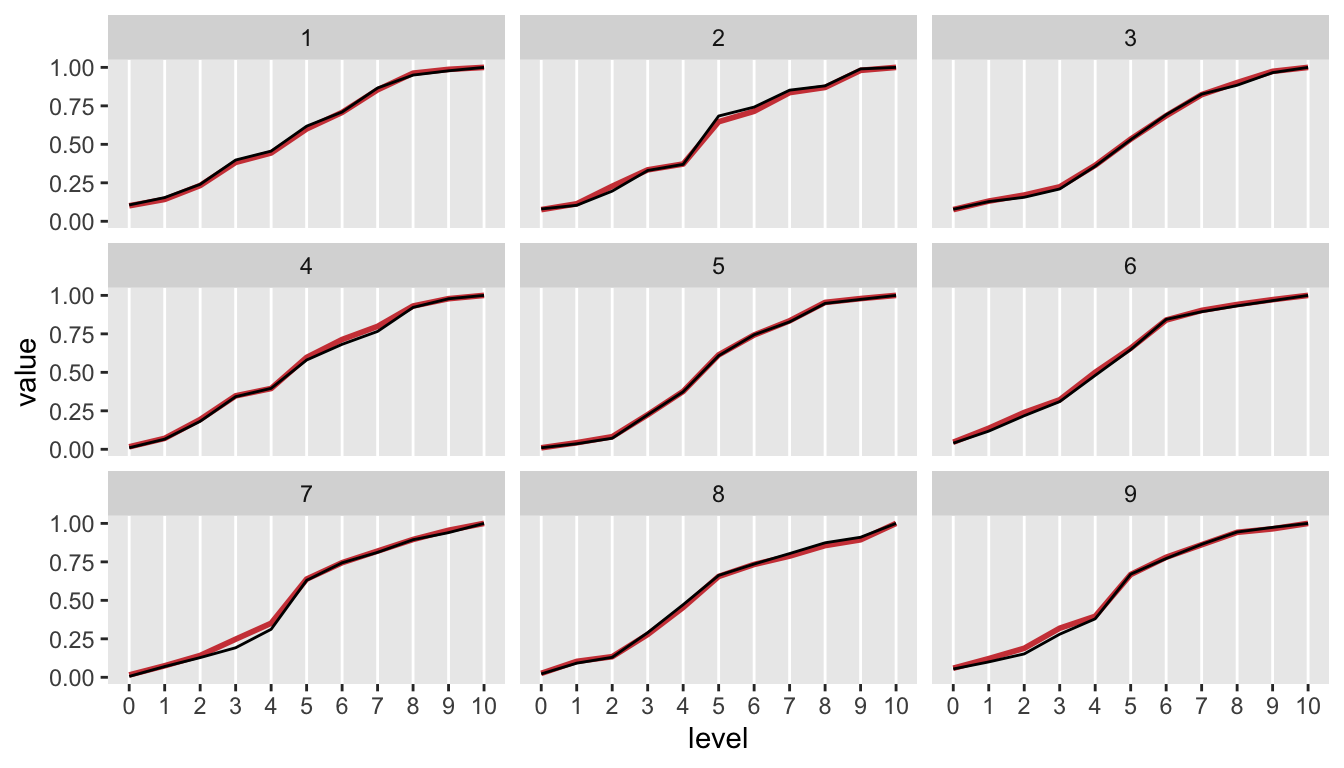
## [9,] 0.054 0.046 0.052 0.128 0.100 0.290 0.102 0.092 0.080 0.030 0.026Of course, the best way to compare is to plot the data for each study. Here is another cumulative probability plot, this time including the observed (generated) probabilities in black over the baseline probabilities used in the data generation in red:
Sometime soon, I plan to incorporate something like the function genBaseProbs into simstudy to make it easier to incorporate non-proportionality assumptions into simulation studies that use ordinal categorical outcomes.
Addendum
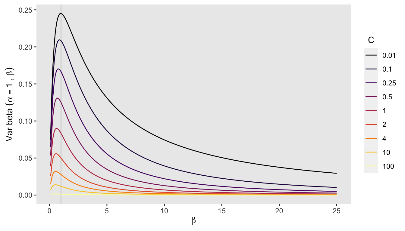
The variance of the beta distribution (and similarly the Dirichlet distribution) decreases as and both increase proportionally (keeping the mean constant). I’ve plotted the variance of the beta distribution for and different levels of and . It is clear that at any level of (I’ve drawn a line at ), the variance decreases as increases. It is also clear that, holding constant, the relationship of to variance is not strictly monotonic:
var_beta <- function(params) {
  a <- params[1]
  b <- params[2]
  (a * b) / ( (a + b)^2 * (a + b + 1))
}

loop_b <- function(C, b) {
  V <- sapply(C, function(x) var_beta(x*c(1, b)))
  data.table(b, V, C)
}

b <- seq(.1, 25, .1)
C <- c(0.01, 0.1, 0.25, 0.5, 1, 2, 4, 10, 100)

d_var <- rbindlist(lapply(b, function(x) loop_b(C, x)))

ggplot(data = d_var, aes(x = b, y = V, group = C)) +
  geom_vline(xintercept = 1, size = .5, color = "grey80") +
  geom_line(aes(color = factor(C))) +
  scale_y_continuous(name = expression("Var beta"~(alpha==1~","~beta))) +
  scale_x_continuous(name = expression(beta)) +
  scale_color_viridis(discrete = TRUE, option = "B", name = "C") +
  theme(panel.grid = element_blank(),
        legend.title.align=0.15)