Here’s the scenario: we have an intervention that we think will improve outcomes for a particular population. Furthermore, there are two sub-groups (let’s say defined by which of two medical conditions each person in the population has) and we are interested in knowing if the intervention effect is different for each sub-group.
And here’s the question: what is the ideal way to set up a study so that we can assess (1) the intervention effects on the group as a whole, but also (2) the sub-group specific intervention effects?
This is a pretty straightforward, text-book scenario. Sub-group analysis is common in many areas of research, including health services research where I do most of my work. It is definitely an advantage to know ahead of time if you want to do a sub-group analysis, as you would in designing a stratified randomized controlled trial. Much of the criticism of these sub-group analyses arises when they are not pre-specified and conducted in an ad hoc manner after the study data have been collected. The danger there, of course, is that the assumptions underlying the validity of a hypothesis test are violated. (It may not be easy to convince folks to avoid hypothesis testing.) In planning ahead for these analyses, researchers are less likely to be accused of snooping through data in search of findings.
So, given that you know you want to do these analyses, the primary issue is how they should be structured. In particular, how should the statistical tests be set up so that we can draw reasonable conclusions? In my mind there are a few ways to answer the question.
Three possible models
Here are three models that can help us assess the effect of an intervention on an outcome in a population with at least two sub-groups:
\[ \text{Model 1: } Y_i = \beta_0 + \beta_1 D_i \]
\[ \text{Model 2: } Y_i = \beta_0^{\prime} + \beta_1^{\prime} D_i + \beta^{\prime}_2 T_i \]
\[ \text{Model 3: } Y_i = \beta_0^{\prime\prime} + \beta_1^{\prime\prime} D_i +\beta^{\prime\prime}_2 T_i +\beta^{\prime\prime}_3 T_i D_i\]
where \(Y_i\) is the outcome for subject \(i\), \(T_i\) is an indicator of treatment and equals 1 if the subject received the treatment, and \(D_i\) is an indicator of having the condition that defines the second sub-group. Model 1 assumes the medical condition can only affect the outcome. Model 2 assumes that if the intervention does have an effect, it is the same regardless of sub-group. And Model 3 allows for the possibility that intervention effects might vary between sub-groups.
1. Main effects
In the first approach, we would estimate both Model 2 and Model 3, and conduct a hypothesis test using the null hypothesis \(\text{H}_{01}\): \(\beta_2^{\prime} = 0\). In this case we would reject \(\text{H}_{01}\) if the p-value for the estimated value of \(\beta_2^{\prime}\) was less than 0.05. If in fact we do reject \(\text{H}_{01}\) (and conclude that there is an overall main effect), we could then (and only then) proceed to a second hypothesis test of the interaction term in Model 3, testing \(\text{H}_{02}\): \(\beta_3^{\prime\prime} = 0\). In this second test we can also evaluate the test using a cutoff of 0.05, because we only do this test if we reject the first one.
This is not a path typically taken, for reasons we will see at the end when we explore the relative power of each test under different effect size scenarios.
2. Interaction effects
In the second approach, we would also estimate just Models 2 and 3, but would reverse the order of the tests. We would first test for interaction in Model 3: \(\text{H}_{01}\): \(\beta_3^{\prime\prime} = 0\). If we reject \(\text{H}_{01}\) (and conclude that the intervention effects are different across the two sub-groups), we stop there, because we have evidence that the intervention has some sort of effect, and that it is different across the sub-groups. (Of course, we can report the point estimates.) However, if we fail to reject \(\text{H}_{01}\), we would proceed to test the main effect from Model 2. In this case we would test \(\text{H}_{02}\): \(\beta_2^{\prime} = 0\).
In this approach, we are forced to adjust the size of our tests (and use, for example, 0.025 as a cutoff for both). Here is a little intuition for why. If we use a cutoff of 0.05 for the first test and in fact there is no effect, 5% of the time we will draw the wrong conclusion (by wrongly rejecting \(\text{H}_{01}\)). However, 95% of the time we will correctly fail to reject the (true) null hypothesis in step one, and thus proceed to step two. Of all the times we proceed to the second step (which will be 95% of the time), we will err 5% of the time (again assuming the null is true). So, 95% of the time we will have an additional 5% error due to the second step, for an error rate of 4.75% due to the second test (95% \(\times\) 5%). In total - adding up the errors from steps 1 and 2 - we will draw the wrong conclusion almost 10% of the time. However, if we use a cutoff of 0.025, then we will be wrong 2.5% of the time in step 1, and about 2.4% (97.5% \(\times\) 2.5%) of the time in the second step, for a total error rate of just under 5%.
In the first approach (looking at the main effect first), we need to make no adjustment, because we only do the second test when we’ve rejected (incorrectly) the null hypothesis. By definition, errors we make in the second step will only occur in cases where we have made an error in the first step. In the first approach where we evaluate main effects first, the errors are nested. In the second, they are not nested but additive.
3. Global test
In the third and last approach, we start by comparing Model 3 with Model 1 using a global F-test. In this case, we are asking the question of whether or not a model that includes treatment as a predictor does “better” than a model that only adjust for sub-group membership. The null hypothesis can crudely be stated as \(\text{H}_{01}\): \(\text{Model }3 = \text{Model }1\). If we reject this hypothesis (and conclude that the intervention does have some sort of effect, either generally or differentially for each sub-group), then we are free to evaluate Models 2 and 3 to see if the there is a varying affect or not.
Here we can use cutoffs of 0.05 in our hypothesis tests. Again, we only make errors in the second step if we’ve made a mistake in the first step. The errors are nested and not additive.
Simulating error rates
This first simulation shows that the error rates of the three approaches are all approximately 5% under the assumption of no intervention effect. That is, given that there is no effect of the intervention on either sub-group (on average), we will draw the wrong conclusion about 5% of the time. In these simulations, the outcome depends only on disease status and not the treatment. Or, in other words, the null hypothesis is in fact true:
library(simstudy)

# define the data

def <- defData(varname = "disease", formula = .5, dist = "binary")

# outcome depends only on sub-group status, not intervention

def2 <- defCondition(condition = "disease == 0",
                     formula = 0.0, variance = 1,
                     dist = "normal")

def2 <- defCondition(def2, condition = "disease == 1",
                     formula = 0.5, variance = 1,
                     dist = "normal")

set.seed(1987) # the year I graduated from college, in case
               # you are wondering ...

pvals <- data.table() # store simulation results

# run 2500 simulations

for (i in 1: 2500) {

  # generate data set

  dx <- genData(400, def)
  dx <- trtAssign(dx, nTrt = 2, balanced = TRUE,
                  strata = "disease", grpName = "trt")

  dx <- addCondition(def2, dx, "y")

  # fit 3 models

  lm1 <- lm(y ~ disease, data = dx)
  lm2 <- lm(y ~ disease + trt, data = dx)
  lm3 <- lm(y ~ disease + trt + trt*disease, data = dx)

  # extract relevant p-values

  cM <- coef(summary(lm2))["trt", 4]
  cI <- coef(summary(lm3))["disease:trt", 4]
  fI <- anova(lm1, lm3)$`Pr(>F)`[2]

  # store the p-values from each iteration

  pvals <- rbind(pvals, data.table(cM, cI, fI))

}

pvals
## cM cI fI
## 1: 0.72272413 0.727465073 0.883669625
## 2: 0.20230262 0.243850267 0.224974909
## 3: 0.83602639 0.897635326 0.970757254
## 4: 0.70949192 0.150259496 0.331072131
## 5: 0.85990787 0.449130976 0.739087609
## ---
## 2496: 0.76142389 0.000834619 0.003572901
## 2497: 0.03942419 0.590363493 0.103971344
## 2498: 0.16305568 0.757882365 0.360893205
## 2499: 0.81873930 0.004805028 0.018188997
## 2500: 0.69122281 0.644801480 0.830958227# Approach 1
pvals[, mEffect := (cM <= 0.05)] # cases where we would reject null
pvals[, iEffect := (cI <= 0.05)]
# total error rate
pvals[, mean(mEffect & iEffect)] +
pvals[, mean(mEffect & !iEffect)]## [1] 0.0496# Approach 2
pvals[, iEffect := (cI <= 0.025)]
pvals[, mEffect := (cM <= 0.025)]
# total error rate
pvals[, mean(iEffect)] +
pvals[, mean((!iEffect) & mEffect)]## [1] 0.054# Approach 3
pvals[, fEffect := (fI <= 0.05)]
pvals[, iEffect := (cI <= 0.05)]
pvals[, mEffect := (cM <= 0.05)]
# total error rate
pvals[, mean(fEffect & iEffect)] +
pvals[, mean(fEffect & !(iEffect) & mEffect)]## [1] 0.05If we use a cutoff of 0.05 for the second approach, we can see that the overall error rate is indeed inflated to close to 10%:
# Approach 2 - with invalid cutoff

pvals[, iEffect := (cI <= 0.05)]
pvals[, mEffect := (cM <= 0.05)]

# total error rate

pvals[, mean(iEffect)] +
  pvals[, mean((!iEffect) & mEffect)]
## [1] 0.1028Exploring power
Now that we have established at least three valid testing schemes, we can compare them by assessing the power of the tests. For the uninitiated, power is simply the probability of concluding that there is an effect when in fact there truly is an effect. Power depends on a number of factors, such as sample size, effect size, variation, and importantly for this post, the testing scheme.
The plot below shows the results of estimating power using a range of assumptions about an intervention’s effect in the two subgroups and the different approaches to testing. (The sample size and variation were fixed across all simulations.) The effect sizes ranged from -0.5 to +0.5. (I have not included the code here, because it is quite similar to what I did to assess the error rates. If anyone wants it, please let me know, and I can post it on github or send it to you.)
The estimated power reflects the probability that the tests correctly rejected at least one null hypothesis. So, if there was no interaction (say both group effects were +0.5) but there was a main effect, we would be correct if we rejected the hypothesis associated with the main effect. Take a look a the plot:
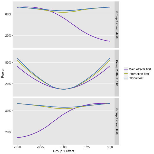
What can we glean from this power simulation? Well, it looks like the global test that compares the interaction model with the null model (Approach 3) is the way to go, but just barely when compared to the approach that focuses solely on the interaction model first.
And, we see clearly that the first approach suffers from a fatal flaw. When the sub-group effects are offsetting, as they are when the effect is -0.5 in subgroup 1 and +0.5 in subgroup 2, we will fail to reject the null that says there is no main effect. As a result, we will never test for interaction and see that in fact the intervention does have an effect on both sub-groups (one positive and one negative). We don’t get to test for interaction, because the rule was designed to keep the error rate at 5% when in fact there is no effect, main or otherwise.
Of course, things are not totally clear cut. If we are quite certain that the effects are going to be positive for both groups, the second approach is not such a disaster. In fact, if we suspect that one of the sub-group effects will be large, it may be preferable to go with this approach. (Look at the right-hand side of the bottom plot to see this.) But, it is still hard to argue (though please do if you feel so inclined), at least based on the assumptions I used in the simulation, that we should take any approach other than the global test.