I’ve been meaning to share an analysis I recently did to estimate the strength of the relationship between a young child’s ability to recognize emotions in others (e.g. teachers and fellow students) and her longer term academic success. The study itself is quite interesting (hopefully it will be published sometime soon), but I really wanted to write about it here as it involved the challenging problem of missing data in the context of heterogeneous effects (different across sub-groups) and clustering (by schools).
As I started to develop simulations to highlight key issues, I found myself getting bogged down in the data generation process. Once I realized I needed to be systematic about thinking how to generate various types of missingness, I thought maybe DAGs would help to clarify some of the issues (I’ve written a bit about DAGS before and provided some links to some good references). I figured that I probably wasn’t the first to think of this, and a quick search confirmed that there is indeed a pretty rich literature on the topic. I first found this blog post by Jake Westfall, which, in addition to describing many of the key issues that I want to address here, provides some excellent references, including this paper by Daniel et al and this one by Mohan et al.
I think the value I can add here is to provide some basic code to get the data generation processes going, in case you want to explore missing data methods for yourself.
Thinking systematically about missingness
In the world of missing data, it has proved to be immensely useful to classify different types of missing data. That is, there could various explanations of how the missingness came to be in a particular data set. This is important, because as in any other modeling problem, having an idea about the data generation process (in this case the missingness generation process) informs how you should proceed to get the “best” estimate possible using the data at hand.
Missingness can be recorded as a binary characteristic of a particular data point for a particular individual; the data point is missing or it is not. It seems to be the convention that the missingness indicator is \(R_{p}\) (where \(p\) is the variable), and \(R_{p} = 1\) if the data point \(p\) is missing and is \(0\) otherwise.
We say data are missing completely at random (MCAR) when \(P(R)\) is independent of all data, observed and missing. For example, if missingness depends on the flip of a coin, the data would be MCAR. Data are missing at random when \(P(R \ | \ D_{obs})\) is independent of \(D_{mis},\) the missing data. In this case, if older people tend to have more missing data, and we’ve recorded age, then the data are MAR. And finally, data are missing not at random (MNAR) when \(P(R \ | \ D_{obs}) = f(D_{mis})\), or missingness is related to the unobserved data even after conditioning on observed data. If missingness is related to the health of a person at follow-up and the outcome measurement reflects the health of a person, then the data are MNAR.
The missingness taxonomy in 3 DAGs
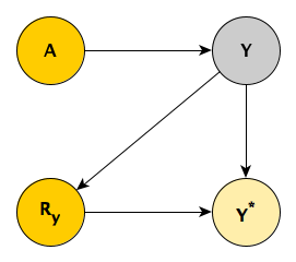
The Mohan et al paper suggests including the missing indicator \(R_p\) directly in the DAG to clarify the nature of dependence between the variables and the missingness. If we have missingness in the outcome \(Y\) (so that for at least one individual \(R_y = 1\)), there is an induced observed variable \(Y^*\) that equals \(Y\) if \(R_y = 0\), and is missing if \(R_y = 1\). \(Y\) represents the complete outcome data, which we don’t observe if there is any missingness. The question is, can we estimate the joint distribution \(P(A, Y)\) (or really any characteristic of the distribution, such as the mean of \(Y\) at different levels of \(A\), which would give us a measure of causal effect) using the observed data \((A, R_y, Y^*)\)? (For much of what follows, I am drawing directly from the Mohan et al paper.)
MCAR
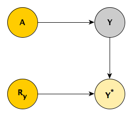
First, consider when the missingness is MCAR, as depicted above. From the DAG, \(A \cup Y \perp \! \! \! \perp R_y\), since \(Y^*\) is a “collider”. It follows that \(P(A, Y) = P(A, Y \ | \ R_y)\), or more specifically \(P(A, Y) = P(A, Y \ | \ R_y=0)\). And when \(R_y = 0\), by definition \(Y = Y^*\). So we end up with \(P(A, Y) = P(A, Y^* \ | \ R_y = 0)\). Using observed data only, we can “recover” the underlying relationship between \(A\) and \(Y\).
A simulation my help to see this. First, we use the simstudy functions to define both the data generation and missing data processes:
def <- defData(varname = "a", formula = 0, variance = 1, dist = "normal")
def <- defData(def, "y", formula = "1*a", variance = 1, dist = "normal")

defM <- defMiss(varname = "y", formula = 0.2, logit.link = FALSE)
The complete data are generated first, followed by the missing data matrix, and ending with the observed data set.
set.seed(983987)

dcomp <- genData(1000, def)
dmiss <- genMiss(dcomp, defM, idvars = "id")
dobs <- genObs(dcomp, dmiss, "id")

head(dobs)
## id a y
## 1: 1 0.171 0.84
## 2: 2 -0.882 0.37
## 3: 3 0.362 NA
## 4: 4 1.951 1.62
## 5: 5 0.069 -0.18
## 6: 6 -2.423 -1.29In this replication, about 22% of the \(Y\) values are missing:
dmiss[, mean(y)]## [1] 0.22If \(P(A, Y) = P(A, Y^* \ | \ R_y = 0)\), then we would expect that the mean of \(Y\) in the complete data set will equal the mean of \(Y^*\) in the observed data set. And indeed, they appear quite close:
round(c(dcomp[, mean(y)], dobs[, mean(y, na.rm = TRUE)]), 2)## [1] 0.03 0.02Going beyond the mean, we can characterize the joint distribution of \(A\) and \(Y\) using a linear model (which we know is true, since that is how we generated the data). Since the outcome data are missing completely at random, we would expect that the relationship between \(A\) and \(Y^*\) to be very close to the true relationship represented by the complete (and not fully observed) data.
fit.comp <- lm(y ~ a, data = dcomp)
fit.obs <- lm(y ~ a, data = dobs)

broom::tidy(fit.comp)
## # A tibble: 2 x 5
## term estimate std.error statistic p.value
## <chr> <dbl> <dbl> <dbl> <dbl>
## 1 (Intercept) -0.00453 0.0314 -0.144 8.85e- 1
## 2 a 0.964 0.0313 30.9 2.62e-147broom::tidy(fit.obs)## # A tibble: 2 x 5
## term estimate std.error statistic p.value
## <chr> <dbl> <dbl> <dbl> <dbl>
## 1 (Intercept) -0.0343 0.0353 -0.969 3.33e- 1
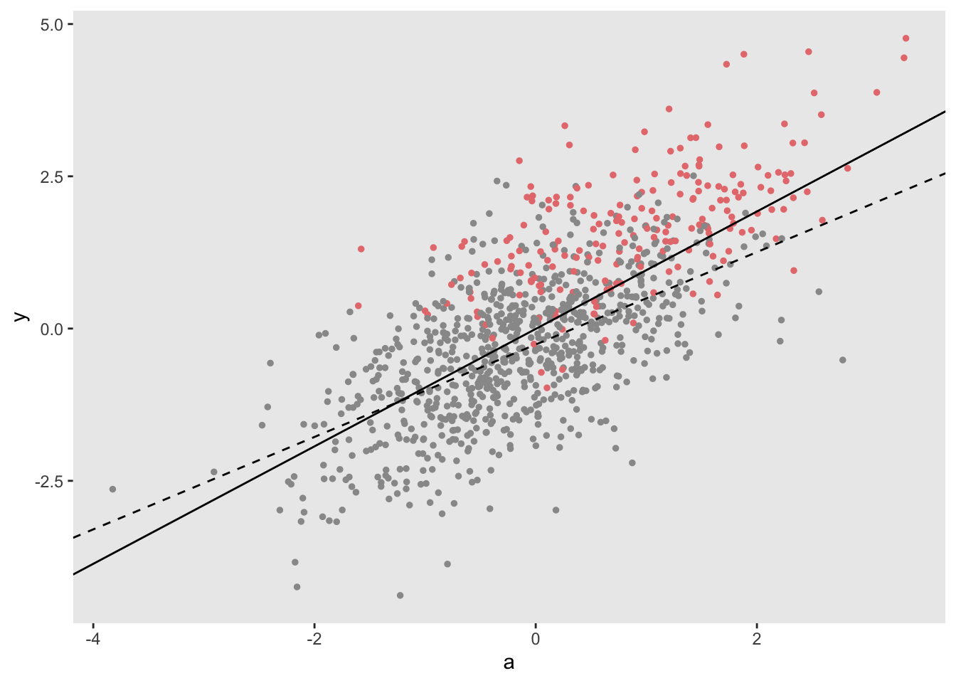
## 2 a 0.954 0.0348 27.4 4.49e-116And if we plot those lines over the actual data, they should be quite close, if not overlapping. In the plot below, the red points represent the true values of the missing data. We can see that missingness is scattered randomly across values of \(A\) and \(Y\) - this is what MCAR data looks like. The solid line represents the fitted regression line based on the full data set (assuming no data are missing) and the dotted line represents the fitted regression line using complete cases only.
dplot <- cbind(dcomp, y.miss = dmiss$y)
ggplot(data = dplot, aes(x = a, y = y)) +
geom_point(aes(color = factor(y.miss)), size = 1) +
scale_color_manual(values = c("grey60", "#e67c7c")) +
geom_abline(intercept = coef(fit.comp)[1],
slope = coef(fit.comp)[2]) +
geom_abline(intercept = coef(fit.obs)[1],
slope = coef(fit.obs)[2], lty = 2) +
theme(legend.position = "none",
panel.grid = element_blank())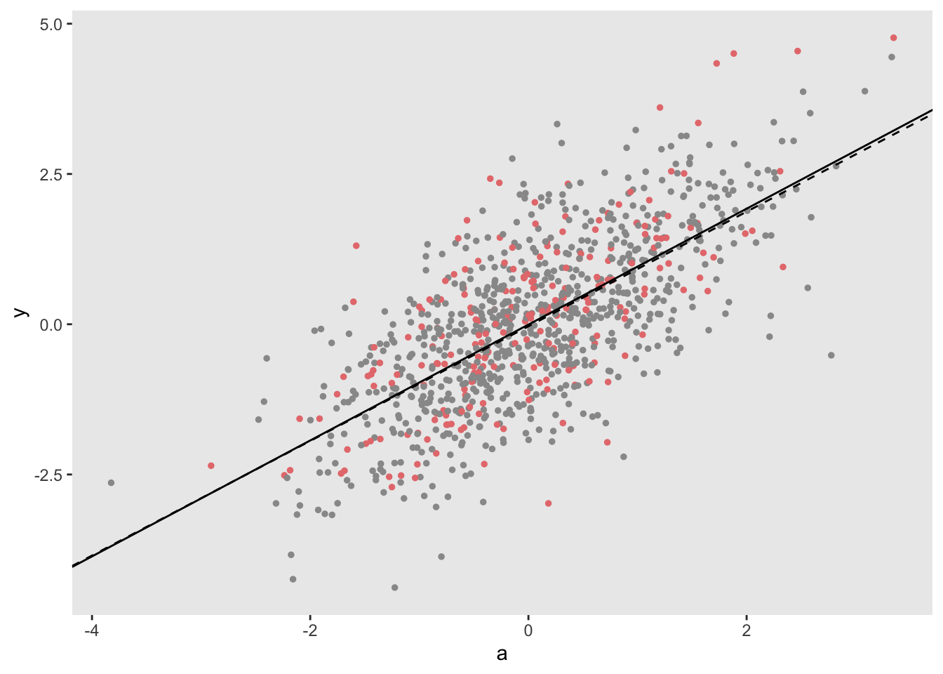
MAR
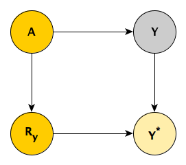
This DAG is showing a MAR pattern, where \(Y \perp \! \! \! \perp R_y \ | \ A\), again because \(Y^*\) is a collider. This means that \(P(Y | A) = P(Y | A, R_y)\). If we decompose \(P(A, Y) = P(Y | A)P(A)\), you can see how that independence is useful. Substituting \(P(Y | A, R_y)\) for \(P(Y | A)\) , \(P(A, Y) = P(Y | A, R_y)P(A)\). Going further, \(P(A, Y) = P(Y | A, R_y=0)P(A)\), which is equal to \(P(Y^* | A, R_y=0)P(A)\). Everything in this last decomposition is observable - \(P(A)\) from the full data set and \(P(Y^* | A, R_y=0)\) from the records with observed \(Y\)’s only.
This implies that, conceptually at least, we can estimate the conditional probability distribution of observed-only \(Y\)’s for each level of \(A\), and then pool the distributions across the fully observed distribution of \(A\). That is, under an assumption of data MAR, we can recover the joint distribution of the full data using observed data only.
To simulate, we keep the data generation process the same as under MCAR; the only thing that changes is the missingness generation process. \(P(R_y)\) now depends on \(A\):
defM <- defMiss(varname = "y", formula = "-2 + 1.5*a", logit.link = TRUE)After generating the data as before, the proportion of missingness is unchanged (though the pattern of missingness certainly is):
dmiss[, mean(y)]## [1] 0.22We do not expect the marginal distribution of \(Y\) and \(Y^*\) to be the same (only the distributions conditional on \(A\) are close), so the means should be different:
round(c(dcomp[, mean(y)], dobs[, mean(y, na.rm = TRUE)]), 2)## [1] 0.03 -0.22However, since the conditional distribution of \((Y|A)\) is equivalent to \((Y^*|A, R_y = 0)\), we would expect estimates from a regression model of \(E[Y] = \beta_0 + \beta_1A)\) would yield estimates very close to \(E[Y^*] = \beta_0^{*} + \beta_1^{*}A\). That is, we would expect \(\beta_1^{*} \approx \beta_1\).
## # A tibble: 2 x 5
##   term        estimate std.error statistic   p.value
##   <chr>          <dbl>     <dbl>     <dbl>     <dbl>
## 1 (Intercept) -0.00453    0.0314    -0.144 8.85e-  1
## 2 a 0.964 0.0313 30.9 2.62e-147## # A tibble: 2 x 5
## term estimate std.error statistic p.value
## <chr> <dbl> <dbl> <dbl> <dbl>
## 1 (Intercept) 0.00756 0.0369 0.205 8.37e- 1
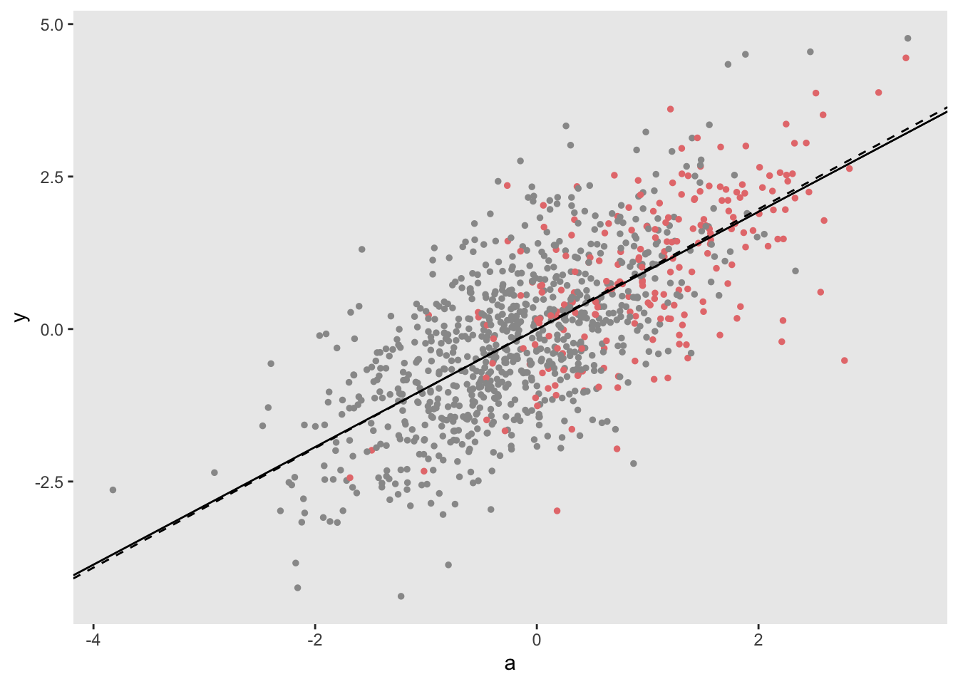
## 2 a 0.980 0.0410 23.9 3.57e-95The overlapping lines in the plot confirm the close model estimates. In addition, you can see here that missingness is associated with higher values of \(A\).
MNAR
In MNAR, there is no way to separate \(Y\) from \(R_y\). Reading from the DAG, \(P(Y) \neq P(Y^* | R_y),\) and \(P(Y|A) \neq P(Y^* | A, R_y),\) There is no way to recover the joint probability of \(P(A,Y)\) with observed data. Mohan et al do show that under some circumstances, it is possible to use observed data to recover the true distribution under MNAR (particularly when there is missingness related to the exposure measurement \(A\)), but not in this particular case.
Daniel et al have a different approach to determine whether the causal relationship of \(A\) and \(Y\) is identifiable under the different mechanisms. They do not use a variable like \(Y^*\), but introduce external nodes \(U_a\) and \(U_y\) representing unmeasured variability related to both exposure and outcome (panel a of the diagram below).
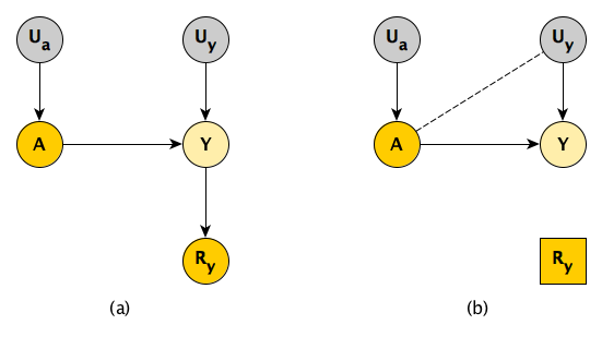
In the case of MNAR, when you use complete cases only, you are effectively controlling for \(R_y\) (panel b). Since \(Y\) is a collider (and \(U_y\) is an ancestor of \(Y\)), this has the effect of inducing an association between \(A\) and \(U_y\), the common causes of \(Y\). By doing this, we have introduced unmeasured confounding that cannot be corrected, because \(U_y\), by definition, always represents the portion of unmeasured variation of \(Y\).
In the simulation, I explicitly generate \(U_y\), so we can see if we observe this association:
def <- defData(varname = "a", formula = 0, variance = 1, dist = "normal")
def <- defData(def, "u.y", formula = 0, variance = 1, dist = "normal")
def <- defData(def, "y", formula = "1*a + u.y", dist = "nonrandom")
This time around, we generate missingness of \(Y\) as a function of \(Y\) itself:
defM <- defMiss(varname = "y", formula = "-3 + 2*y", logit.link = TRUE)And this results in just over 20% missingness:
dmiss[, mean(y)]## [1] 0.21Indeed, \(A\) and \(U_y\) are virtually uncorrelated in the full data set, but are negatively correlated in the cases where \(Y\) is not missing, as theory would suggest:
round(c(dcomp[, cor(a, u.y)], dobs[!is.na(y), cor(a, u.y)]), 2)## [1] -0.04 -0.23The plot generated from these data shows diverging regression lines, the divergence a result of the induced unmeasured confounding.
In this MNAR example, we see that the missingness is indeed associated with higher values of \(Y\), although the proportion of missingness remains at about 21%, consistent with the earlier simulations.
There may be more down the road
I’ll close here, but in the near future, I hope to explore various (slightly more involved) scenarios under which complete case analysis is adequate, or where something like multiple imputation is more useful. Also, I would like to get back to the original motivation for writing about missingness, which was to describe how I went about analyzing the child emotional intelligence data. Both of these will be much easier now that we have the basic tools to think about how missing data can be generated in a systematic way.
References:
Daniel, Rhian M., Michael G. Kenward, Simon N. Cousens, and Bianca L. De Stavola. “Using causal diagrams to guide analysis in missing data problems.” Statistical methods in medical research 21, no. 3 (2012): 243-256.
Mohan, Karthika, Judea Pearl, and Jin Tian. “Graphical models for inference with missing data.” In Advances in neural information processing systems, pp. 1277-1285. 2013.
Westfall, Jake. “Using causal graphs to understand missingness and how to deal with it.” Cookie Scientist (blog). August 22, 2017. Accessed March 25, 2019. http://jakewestfall.org/blog/.