Even with randomization, mediation analysis can still be confounded

Randomization is super useful because it usually eliminates the risk that confounding will lead to a biased estimate of a treatment effect. However, this only goes so far. If you are conducting a meditation analysis in the hopes of understanding the underlying causal mechanism of a treatment, it is important to remember that the mediator has not been randomized, only the treatment. This means that the estimated mediation effect is still at risk of being confounded.

I never fail to mention this when a researcher tells me they are interested in doing a mediation analysis (and it seems like more and more folks are interested in including this analysis as part of their studies). So, when my son brought up the fact that the lead investigator on his experimental psychology project wanted to include a mediation analysis, I, of course, had to pipe up. “You have to be careful, you know.”

But, he wasn’t buying it, wondering why randomization didn’t take care of the confounding; surely, the potential confounders would be balanced across treatment groups. Maybe I’d had a little too much wine, as I considered he might have a point. But no - I’d quickly come to my senses - it doesn’t matter that the confounder is balanced across treatment groups (which it very well could be), it would still be unbalanced across the different levels of the mediator, which is what really matters if we are estimating the effect of the mediator.

I proposed to do a simulation of this phenomenon. My son was not impressed, but I went ahead and did it anyways, and I am saving it here in case he wants to take a look. Incidentally, this is effectively a brief follow-up to an earlier post on mediation. So, if the way in which I am generating the data seems a bit opaque, you might want to take a look at what I did earlier.

The data generating process

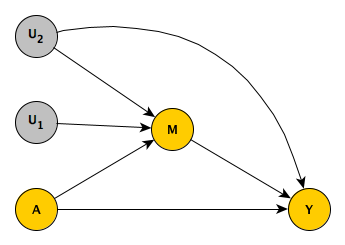
Here is a DAG that succinctly describes how I will generate the data. You can see clearly that \(U_2\) is a confounder of the relationship between the mediator \(M\) and the outcome \(Y\). (It should be noted that if we were only interested in is the causal effect of \(A\) on \(Y\), \(U_2\) is not a confounder, so we wouldn’t need to control for \(U_2\).)

As I did in the earlier simulation of mediation, I am simulating the potential outcomes so that we can see the “truth” that we are trying to measure.

defU <- defData(varname = "U2", formula = 0, 
                variance = 1.5, dist = "normal")

defI <- defDataAdd(varname = "M0", formula = "-2 + U2",
                   dist = "binary", link = "logit")
defI <- defDataAdd(defI, varname = "M1", formula = "-1 + U2",
                   dist = "binary", link = "logit")

defA <- defReadAdd("DataConfoundMediation/mediation def.csv")

varname	formula	variance	dist	link
e0	0	1	normal	identity
Y0M0	2 + M0*2 + U2 + e0	0	nonrandom	identity
Y0M1	2 + M1*2 + U2 + e0	0	nonrandom	identity
e1	0	1	normal	identity
Y1M0	8 + M0*5 + U2 + e1	0	nonrandom	identity
Y1M1	8 + M1*5 + U2 + e1	0	nonrandom	identity
M	(A==0) * M0 + (A==1) * M1	0	nonrandom	identity
Y	(A==0) * Y0M0 + (A==1) * Y1M1	0	nonrandom	identity

Getting the “true”" causal effects

With the definitions set, we can generate a very, very large data set (not infinite, but pretty close) to get at the “true” causal effects that we will try to recover using smaller (finite) data sets. I am calculating the causal mediated effects (for the treated and controls) and the causal direct effects (also for the treated and controls).

set.seed(184049)

du <- genData(1000000, defU)
dtrue <- addCorFlex(du, defI, rho = 0.6, corstr = "cs")

dtrue <- trtAssign(dtrue, grpName = "A")

dtrue <- addColumns(defA, dtrue)

truth <- round(dtrue[, .(CMEc = mean(Y0M1 - Y0M0), CMEt= mean(Y1M1 - Y1M0),
                  CDEc = mean(Y1M0 - Y0M0), CDEt= mean(Y1M1 - Y0M1))], 2)

truth

##    CMEc CMEt CDEc CDEt
## 1: 0.29 0.72 6.51 6.95

And here we can see that although \(U_2\) is balanced across treatment groups \(A\), \(U_2\) is still associated with the mediator \(M\):

dtrue[, mean(U2), keyby = A]

##    A       V1
## 1: 0 -0.00220
## 2: 1 -0.00326

dtrue[, mean(U2), keyby = M]

##    M     V1
## 1: 0 -0.287
## 2: 1  0.884

Also - since \(U_2\) is a confounder, we would expect it to be associated with the outcome \(Y\), which it is:

dtrue[, cor(U2, Y)]

## [1] 0.42

Recovering the estimate from a small data set

We generate a smaller data set using the same process:

du <- genData(1000, defU)
dd <- addCorFlex(du, defI, rho = 0.6, corstr = "cs")
dd <- trtAssign(dd, grpName = "A")
dd <- addColumns(defA,dd)

We can estimate the causal effects using the mediation package, by specifying a “mediation” model and an “outcome model”. I am going to compare two approaches, one that controls for \(U_2\) in both models, and a second that ignores the confounder in both.

library(mediation)

### models that control for confounder

med.fitc <- glm(M ~ A + U2, data = dd, family = binomial("logit"))
out.fitc <- lm(Y ~ M*A + U2, data = dd)

med.outc <- mediate(med.fitc, out.fitc, treat = "A", mediator = "M",
                   robustSE = TRUE, sims = 500)

### models that ignore confounder

med.fitx <- glm(M ~ A, data = dd, family = binomial("logit"))
out.fitx <- lm(Y ~ M*A, data = dd)

med.outx <- mediate(med.fitx, out.fitx, treat = "A", mediator = "M",
                   robustSE = TRUE, sims = 500)

It appears that the approach that adjusts for \(U_2\) (middle row) provides a set of estimates closer to the truth (top row) than the approach that ignores \(U_2\) (bottom row):

dres <- rbind(
  
  truth,

  data.table(CMEc = med.outc$d0, CMEt = med.outc$d1, 
             CDEc = med.outc$z0, CDEt = med.outc$z1) ,

  data.table(CMEc = med.outx$d0, CMEt = med.outx$d1, 
             CDEc = med.outx$z0, CDEt = med.outx$z1)
)

round(dres,2)

##    CMEc CMEt CDEc CDEt
## 1: 0.29 0.72 6.51 6.95
## 2: 0.32 0.84 6.51 7.03
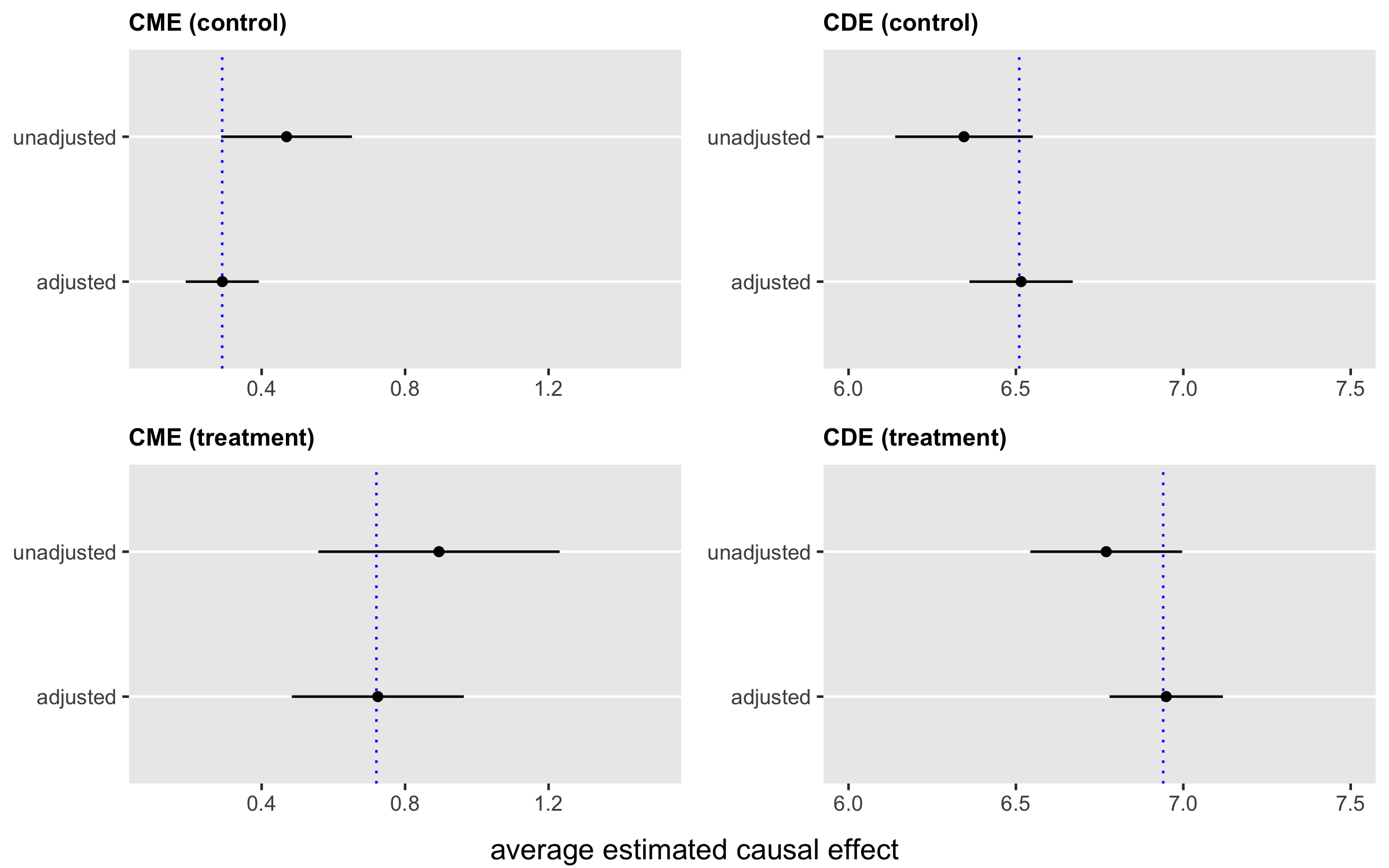
## 3: 0.53 1.07 6.32 6.85

Of course, it is not prudent to draw conclusions from a single simulation. So, I generated 1000 data sets and recorded all the results. A visual summary of the results shows that the approach that ignores \(U_2\) is biased with respect to the four causal effects, whereas including \(U_2\) in the analysis yields unbiased estimates. In the plot, the averages of the estimates are the black points, the segments represent \(\pm \ 2 \ sd\), and the blue vertical lines represent the truth:

Almost as an addendum, using the almost infinitely large “true” data set, we can see that the total treatment effect of \(A\) can be estimated from observed data ignoring \(U_2\), because as we saw earlier, \(U_2\) is indeed balanced across both levels of \(A\) due to randomization:

c( est = coef(lm(Y ~ A, data = dtrue))["A"], 
   truth = round(dtrue[, .(TotalEff = mean(Y1M1 - Y0M0))], 2))

## $est.A
## [1] 7.24
## 
## $truth.TotalEff
## [1] 7.24