Towards the end of Part 1 of this short series on confounding, IPW, and (hopefully) marginal structural models, I talked a little bit about the fact that inverse probability weighting (IPW) can provide unbiased estimates of marginal causal effects in the context of confounding just as more traditional regression models like OLS can. I used an example based on a normally distributed outcome. Now, that example wasn’t super interesting, because in the case of a linear model with homogeneous treatment effects (i.e. no interaction), the marginal causal effect is the same as the conditional effect (that is, conditional on the confounders.) There was no real reason to use IPW in that example - I just wanted to illustrate that the estimates looked reasonable.
But in many cases, the conditional effect is different from the marginal effect. (And in other cases, there may not even be an obvious way to estimate the conditional effect - that will be the topic for the last post in this series). When the outcome is binary, the notion that conditional effects are equal to marginal effects is no longer the case. (I’ve touched on this before.) What this means, is that we can recover the true conditional effects using logistic regression, but we cannot estimate the marginal effect. This is directly related to the fact that logistic regression is linear on the logit (or log-odds) scale, not on the probability scale. The issue here is collapsibility, or rather, non-collapsibility.
A simulation
Because binary outcomes are less amenable to visual illustration, I am going to stick with model estimation to see how this plays out:
library(simstudy)

# define the data

defB <- defData(varname = "L", formula =0.27,
                dist = "binary")
defB <- defData(defB, varname = "Y0", formula = "-2.5 + 1.75*L",
                dist = "binary", link = "logit")
defB <- defData(defB, varname = "Y1", formula = "-1.5 + 1.75*L",
                dist = "binary", link = "logit")
defB <- defData(defB, varname = "A", formula = "0.315 + 0.352 * L",
                dist = "binary")
defB <- defData(defB, varname = "Y", formula = "Y0 + A * (Y1 - Y0)",
                dist = "nonrandom")

# generate the data

set.seed(2002)
dtB <- genData(200000, defB)
dtB[1:6]
## id L Y0 Y1 A Y
## 1: 1 0 0 0 0 0
## 2: 2 0 0 0 0 0
## 3: 3 1 0 1 1 1
## 4: 4 0 1 1 1 1
## 5: 5 1 0 0 1 0
## 6: 6 1 0 0 0 0We can look directly at the potential outcomes to see the true causal effect, measured as a log odds ratio (LOR):
odds <- function (p) {
    return((p/(1 - p)))
}

# log odds ratio for entire sample (marginal LOR)

dtB[, log( odds( mean(Y1) ) / odds( mean(Y0) ) )]
## [1] 0.8651611In the linear regression context, the conditional effect measured using observed data from the exposed and unexposed subgroups was in fact a good estimate of the marginal effect in the population. Not the case here, as the conditional causal effect (LOR) of A is 1.0, which is greater than the true marginal effect of 0.86:
library(broom)
tidy(glm(Y ~ A + L , data = dtB, family="binomial"))
## term estimate std.error statistic p.value
## 1 (Intercept) -2.4895846 0.01053398 -236.33836 0
## 2 A 0.9947154 0.01268904 78.39167 0
## 3 L 1.7411358 0.01249180 139.38225 0This regression estimate for the coefficient of \(A\) is a good estimate of the conditional effect in the population (based on the potential outcomes at each level of \(L\)):
dtB[, .(LOR = log( odds( mean(Y1) ) / odds( mean(Y0) ) ) ), keyby = L]## L LOR
## 1: 0 0.9842565
## 2: 1 0.9865561Of course, ignoring the confounder \(L\) is not very useful if we are interested in recovering the marginal effect. The estimate of 1.4 is biased for both the conditional effect and the marginal effect - it is not really useful for anything:
tidy(glm(Y ~ A , data = dtB, family="binomial"))## term estimate std.error statistic p.value
## 1 (Intercept) -2.049994 0.009164085 -223.6987 0
## 2 A 1.433094 0.011723767 122.2384 0How weighting reshapes the data …
Here is a simple tree graph that shows the potential outcomes for 1000 individuals (based on the same distributions we’ve been using in our simulation). For 27% of the individuals, \(L=1\), for 73% \(L=0\). Each individual has a potential outcome under each level of treatment \(A\). So, that is why there are 730 individuals with \(L=0\) who are both with and without treatment. Likewise each treatment arm for those with \(L=0\) has 270 individuals. We are not double counting.
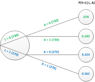
Both the marginal and conditional estimates that we estimated before using the simulated data can be calculated directly using information from this tree. The conditional effects on the log-odds scale can be calculated as …
\[LOR_{A=1 \textbf{ vs } A=0|L = 0} = log \left (\frac{0.182/0.818}{0.076/0.924} \right)=log(2.705) = 0.995\]
and
\[LOR_{A=1 \textbf{ vs } A=0|L = 1} = log \left (\frac{0.562/0.438}{0.324/0.676} \right)=log(2.677) = 0.984\]
The marginal effect on the log odds scale is estimated marginal probabilities: \(P(Y=1|A=0)\) and \(P(Y=1|A=1)\). Again, we can take this right from the tree …
\[P(Y=1|A=0) = 0.73\times0.076 + 0.27\times0.324 = 0.143\] and
\[P(Y=1|A=1) = 0.73\times0.182 + 0.27\times0.562 = 0.285\]
Based on these average outcomes (probabilities) by exposure, the marginal log-odds for the sample is:
\[LOR_{A=1 \textbf{ vs } A=0} = log \left (\frac{0.285/0.715}{0.143/0.857} \right)=log(2.389) = 0.871\]
Back in the real world of observed data, this is what the tree diagram looks like:
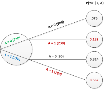
This tree tells us that the probability of exposure \(A=1\) is different depending upon that value of \(L\). For \(L=1\), \(P(A=1) = 230/730 = 0.315\) and for \(L=0\), \(P(A=1) = 180/270 = 0.667\). Because of this disparity, the crude estimate of the effect (ignoring \(L\)) is biased for the marginal causal effect:
\[P(Y=1|A=0) = \frac{500\times0.076 + 90\times0.324}{500+90}=0.114\]
and
\[P(Y=1|A=1) = \frac{230\times0.182 + 180\times0.562}{230+180}=0.349\]
The crude log odds ratio is
\[LOR_{A=1 \textbf{ vs } A=0} = log \left (\frac{0.349/0.651}{0.114/0.886} \right)=log(4.170) = 1.420\]
And now we finally get to the weights. As mentioned in the prior post, the IPW is based on the probability of the actual exposure at each level of \(L\): \(P(A=a | L)\), where \(a\in(0,1)\) (and not on \(P(A=1|L)\), the propensity score). Here are the simple weights for each group:
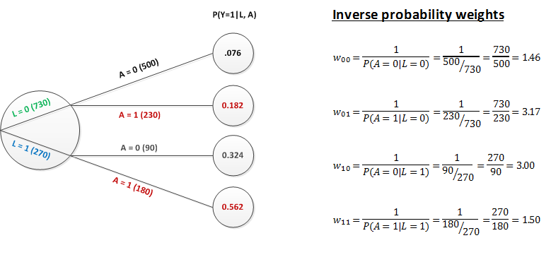
If we apply the weights to each of the respective groups, you can see that the number of individuals in each treatment arm is adjusted to the total number of individuals in the sub-group defined the level of \(L\). For example, if we apply the weight of 3.17 (730/230) to each person observed with \(L=0\) and \(A=1\), we end up with \(230\times3.17=730\). Applying each of the respective weights to the subgroups of \(L\) and \(A\) results in a new sample of individuals that looks exactly like the one we started out with in the potential outcomes world:
This all works only if we make these two assumptions: \[P(Y=1|A=0, L=l) = P(Y_0=1 | A=1, L=l)\] and \[P(Y=1|A=1, L=l) = P(Y_1=1 | A=0, L=l)\]
That is, we can make this claim only under the assumption of no unmeasured confounding. (This was discussed in the Part 1 post.)
Applying IPW to our data
We need to estimate the weights using logistic regression (though other, more flexible methods, can also be used). First, we estimate \(P(A=1|L)\) …
exposureModel <- glm(A ~ L, data = dtB, family = "binomial")
dtB[, pA := predict(exposureModel, type = "response")]
Now we can derive an estimate for \(P(A=a|L=l)\) and get the weight itself…
# Define two new columns
defB2 <- defDataAdd(varname = "pA_actual",
                    formula = "(A * pA) + ((1 - A) * (1 - pA))",
                    dist = "nonrandom")
defB2 <- defDataAdd(defB2, varname = "IPW",
                    formula = "1/pA_actual",
                    dist = "nonrandom")

# Add weights
dtB <- addColumns(defB2, dtB)
dtB[1:6]
## id L Y0 Y1 A Y pA pA_actual IPW
## 1: 1 0 0 0 0 0 0.3146009 0.6853991 1.459004
## 2: 2 0 0 0 0 0 0.3146009 0.6853991 1.459004
## 3: 3 1 0 1 1 1 0.6682351 0.6682351 1.496479
## 4: 4 0 1 1 1 1 0.3146009 0.3146009 3.178631
## 5: 5 1 0 0 1 0 0.6682351 0.6682351 1.496479
## 6: 6 1 0 0 0 0 0.6682351 0.3317649 3.014183To estimate the marginal effect on the log-odds scale, we use the function glm with weights specified by IPW. The true value of marginal effect (based on the population-wide potential outcomes) was 0.87 (as we estimated from the potential outcomes directly and from the tree graph). Our estimate here is spot on (but with such a large sample size, this is not so surprising):
tidy(glm(Y ~ A , data = dtB, family="binomial", weights = IPW)) ## term estimate std.error statistic p.value
## 1 (Intercept) -1.7879512 0.006381189 -280.1909 0
## 2 A 0.8743154 0.008074115 108.2862 0It may not seem like a big deal to be able to estimate the marginal effect - we may actually not be interested in it. However, in the next post, I will touch on the issue of estimating causal effects when there are repeated exposures (for example, administering a drug over time) and time dependent confounders that are both affected by prior exposures and affect future exposures and affect the outcome. Under this scenario, it is very difficult if not impossible to control for these confounders - the best we might be able to do is estimate a marginal, population-wide causal effect. That is where weighting will be really useful.