Way back when I was studying algebra and wrestling with one word problem after another (I think now they call them story problems), I complained to my father. He laughed and told me to get used to it. “Life is one big word problem,” is how he put it. Well, maybe one could say any statistical analysis is really just some form of multilevel data analysis, whether we treat it that way or not.
A key feature of the multilevel model is the ability to explicitly untangle the variation that occurs at different levels. Variation of individuals within a sub-group, variation across sub-groups, variation across groups of sub-groups, and so on. The intra-class coefficient (ICC) is one summarizing statistic that attempts to characterize the relative variability across the different levels.
The amount of clustering as measured by the ICC has implications for study design, because it communicates how much information is available at different levels of the hierarchy. We may have thousands of individuals that fall into ten or twenty clusters, and think we have a lot of information. But if most of the variation is at the cluster/group level (and not across individuals within a cluster), we don’t have thousands of observations, but more like ten or twenty. This has important implications for our measures of uncertainty.
Recently, a researcher was trying to use simstudy to generate cost and quality-of-life measurements to simulate clustered data for a cost-effectiveness analysis. (They wanted the cost and quality measurements to correlate within individuals, but I am going to ignore that aspect here.) Cost data are typically right skewed with most values falling on the lower end, but with some extremely high values on the upper end. (These dollar values cannot be negative.)
Because of this characteristic shape, cost data are often modeled using a Gamma distribution. The challenge here was that in simulating the data, the researcher wanted to control the group level variation relative to the individual-level variation. If the data were normally distributed, it would be natural to talk about that control in terms of the ICC. But, with the Gamma distribution, it is not as obvious how to partition the variation.
As most of my posts do, this one provides simulation and plots to illuminate some of these issues.
Gamma distribtution
The Gamma distribution is a continuous probability distribution that includes all non-negative numbers. The probability density function is typically written as a function of two parameters - the shape \(\alpha\) and the rate \(\beta\):
\[f(x) = \frac{\beta ^ \alpha}{\Gamma(\alpha)} x^{\alpha - 1} e^{-\beta x},\]
with \(\text{E}(x) = \alpha / \beta\), and \(\text{Var}(x)=\alpha / \beta^2\). \(\Gamma(.)\) is the continuous Gamma function, which lends its name to the distribution. (When \(\alpha\) is a positive integer, \(\Gamma(\alpha)=(\alpha - 1 )!\)) In simstudy, I decided to parameterize the pdf using \(\mu\) to represent the mean and a dispersion parameter \(\nu\), where \(\text{Var}(x) = \nu\mu^2\). In this parameterization, shape \(\alpha = \frac{1}{\nu}\) and rate \(\beta = \frac{1}{\nu\mu}\). (There is a simstudy function gammaGetShapeRate that maps \(\mu\) and \(\nu\) to \(\alpha\) and \(\beta\).) With this parameterization, it is clear that the variance of a Gamma distributed random variable is a function of the (square) of the mean.
Simulating data gives a sense of the shape of the distribution and also makes clear that the variance depends on the mean (which is not the case for the normal distribution):
mu <- 20
nu <- 1.2

# theoretical mean and variance
c(mean = mu, variance = mu^2 * nu)
## mean variance
## 20 480library(simstudy)
(ab <- gammaGetShapeRate(mu, nu))## $shape
## [1] 0.8333333
##
## $rate
## [1] 0.04166667# simulate data using R function
set.seed(1)
g.rfunc <- rgamma(100000, ab$shape, ab$rate)
round(c(mean(g.rfunc), var(g.rfunc)), 2)## [1] 19.97 479.52# simulate data using simstudy function - no difference
set.seed(1)
defg <- defData(varname = "g.sim", formula = mu, variance = nu,
dist = "gamma")
dt.g1 <- genData(100000, defg)
dt.g1[, .(round(mean(g.sim),2), round(var(g.sim),2))]## V1 V2
## 1: 19.97 479.52# doubling dispersion factor
defg <- updateDef(defg, changevar = "g.sim", newvariance = nu * 2)
dt.g0 <- genData(100000, defg)
dt.g0[, .(round(mean(g.sim),2), round(var(g.sim),2))]## V1 V2
## 1: 20.09 983.01# halving dispersion factor
defg <- updateDef(defg, changevar = "g.sim", newvariance = nu * 0.5)
dt.g2 <- genData(100000, defg)
dt.g2[, .(round(mean(g.sim),2), round(var(g.sim),2))]## V1 V2
## 1: 19.98 240.16Generating data sets with the same mean but decreasing levels of dispersion makes it appear as if the distribution is “moving” to the right: the peak shifts to the right and variance decreases …
library(ggplot2)

dt.g0[, nugrp := 0]
dt.g1[, nugrp := 1]
dt.g2[, nugrp := 2]

dt.g <- rbind(dt.g0, dt.g1, dt.g2)

ggplot(data = dt.g, aes(x=g.sim), group = nugrp) +
  geom_density(aes(fill=factor(nugrp)), alpha = .5) +
  scale_fill_manual(values = c("#226ab2","#b22222","#22b26a"),
                    labels = c(nu*2, nu, nu*0.5),
                    name =  bquote(nu)) +
  scale_y_continuous(limits = c(0, 0.10)) +
  scale_x_continuous(limits = c(0, 100)) +
  theme(panel.grid.minor = element_blank()) +
  ggtitle(paste0("Varying dispersion with mean = ", mu))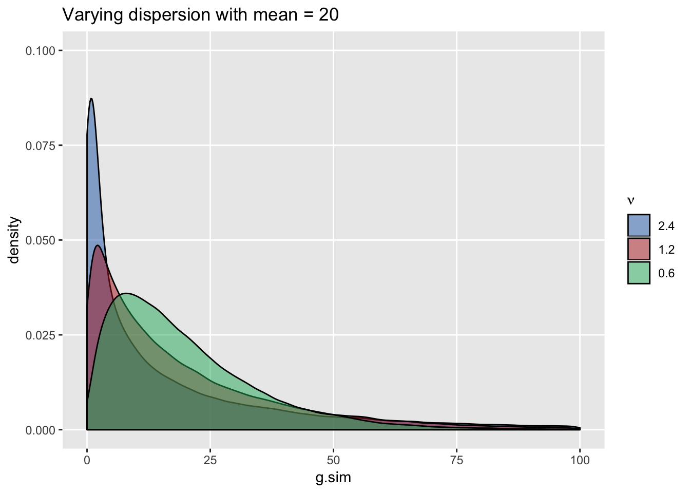
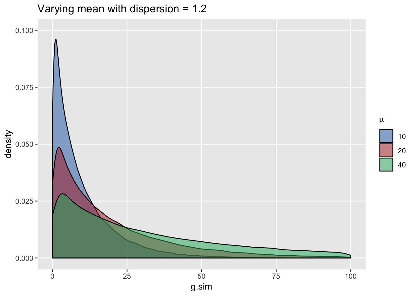
Conversely, generating data with constant dispersion but increasing the mean does not shift the location but makes the distribution appear less “peaked”. In this case, variance increases with higher means (we can see that longer tails are associated with higher means) …
ICC for clustered data where within-group observations have a Gaussian (normal) distribution
In a 2-level world, with multiple groups each containing individuals, a normally distributed continuous outcome can be described by this simple model: \[Y_{ij} = \mu + a_j + e_{ij},\] where \(Y_{ij}\) is the outcome for individual \(i\) who is a member of group \(j\). \(\mu\) is the average across all groups and individuals. \(a_j\) is the group level effect and is typically assumed to be normally distributed as \(N(0, \sigma^2_a)\), and \(e_{ij}\) is the individual level effect that is \(N(0, \sigma^2_e)\). The variance of \(Y_{ij}\) is \(\text{Var}(a_j + e_{ij}) = \text{Var}(a_j) + \text{Var}(e_{ij}) = \sigma^2_a + \sigma^2_e\). The ICC is the proportion of total variation of \(Y\) explained by the group variation: \[ICC = \frac{\sigma^2_a}{\sigma^2_a+\sigma^2_e}\] If individual level variation is relatively low or variation across groups is relatively high, then the ICC will be higher. Conversely, higher individual variation or lower variation between groups implies a smaller ICC.
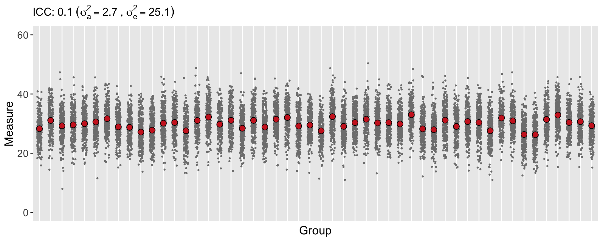
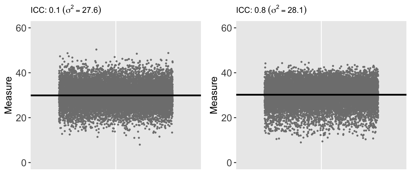
Here is a simulation of data for 50 groups, where each group has 250 individuals. The ICC is 0.10:
# define the group level data

defgrp <- defData(varname = "a", formula = 0,
               variance = 2.8, dist = "normal", id = "cid")
defgrp <- defData(defgrp, varname = "n", formula = 250,
               dist = "nonrandom")

# define the individual level data

defind <- defDataAdd(varname = "ynorm", formula = "30 + a",
                   variance = 25.2, dist = "normal")

# generate the group and individual level data

set.seed(3017)

dt <- genData(50, defgrp)
dc <- genCluster(dt, "cid", "n", "id")
dc <- addColumns(defind, dc)
dc
## cid a n id ynorm
## 1: 1 -2.133488 250 1 30.78689
## 2: 1 -2.133488 250 2 25.48245
## 3: 1 -2.133488 250 3 22.48975
## 4: 1 -2.133488 250 4 30.61370
## 5: 1 -2.133488 250 5 22.51571
## ---
## 12496: 50 -1.294690 250 12496 25.26879
## 12497: 50 -1.294690 250 12497 27.12190
## 12498: 50 -1.294690 250 12498 34.82744
## 12499: 50 -1.294690 250 12499 27.93607
## 12500: 50 -1.294690 250 12500 32.33438# mean Y by group
davg <- dc[, .(avgy = mean(ynorm)), keyby = cid]
# variance of group means
(between.var <- davg[, var(avgy)])## [1] 2.70381# overall (marginal) mean and var of Y
gavg <- dc[, mean(ynorm)]
gvar <- dc[, var(ynorm)]
# individual variance within each group
dvar <- dc[, .(vary = var(ynorm)), keyby = cid]
(within.var <- dvar[, mean(vary)])## [1] 25.08481# estimate of ICC
(ICCest <- between.var/(between.var + within.var))## [1] 0.09729918ggplot(data=dc, aes(y = ynorm, x = factor(cid))) +
geom_jitter(size = .5, color = "grey50", width = 0.2) +
geom_point(data = davg, aes(y = avgy, x = factor(cid)),
shape = 21, fill = "firebrick3", size = 3) +
theme(panel.grid.major.y = element_blank(),
panel.grid.minor.y = element_blank(),
axis.ticks.x = element_blank(),
axis.text.x = element_blank(),
axis.text.y = element_text(size = 12),
axis.title = element_text(size = 14)
) +
xlab("Group") +
scale_y_continuous(limits = c(0, 60), name = "Measure") +
ggtitle(bquote("ICC:" ~ .(round(ICCest, 2)) ~
(sigma[a]^2 == .(round(between.var, 1)) ~ "," ~
sigma[e]^2 == .(round(within.var, 1)))
)) 
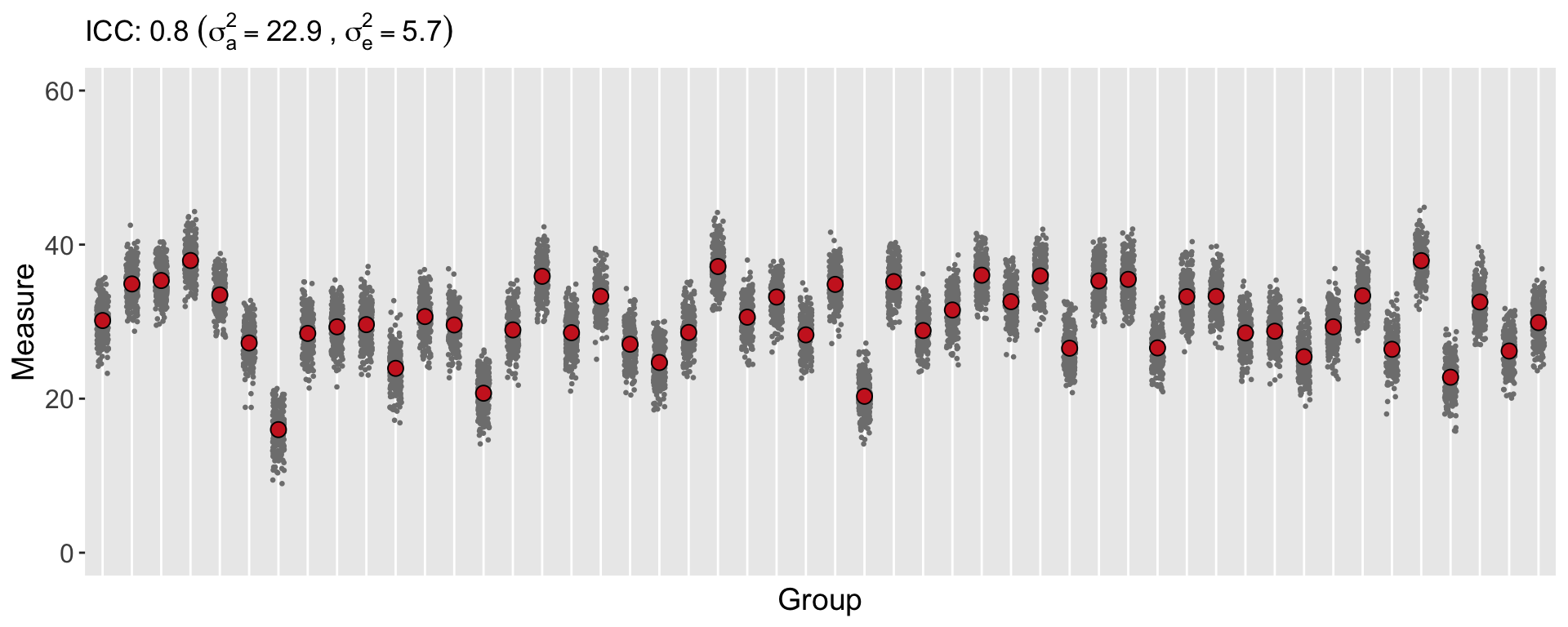
Here is a plot of data generated using the same overall variance of 28, but based on a much higher ICC of 0.80. Almost all of the variation in the data is driven by the clusters rather than the individuals. This has implications for a study, because (in contrast to the first data set generated above) the individual-level data is not providing as much information or insight into the variation of \(Y\). The most useful information (from this extreme example) can be derived from the difference between the groups (so we really have more like 50 data points rather than 125K).
Of course, if we look at the individual-level data for each of the two data sets while ignoring the group membership, the two data sets are indistinguishable. That is, the marginal (or population level) distributions are both normally distributed with mean 30 and variance 28:
ICC for clustered data with Gamma distribution
Now, back to the original question … how do we think about the ICC with clustered data that is Gamma distributed? The model (and data generating process) for these type of data can be described as:
\[Y_{ij} \sim \text{gamma}(\mu_{j}, \nu),\] where \(\text{E}(Y_{j}) = \mu_j\) and \(\text{Var}(Y_j) = \nu\mu_j^2\). In addition, the mean of each group is often modeled as:
\[\text{log}(\mu_j) = \beta + a_j,\] where \(\beta\) is log of the mean for the group whose group effect is 0, and \(a_j \sim N(0, \sigma^2_a)\). So, the group means are normally distributed on the log scale (or are lognormal) with variance \(\sigma^2_a\). (Although the individual observations within each cluster are Gamma-distributed, the means of the groups are not themselves Gamma-distributed.)
But what is the within group (individual) variation, which is Gamma-distributed? It is not so clear, as the variance within each group depends on both the group mean \(\mu_j\) and the dispersion factor \(\nu\). A paper by Nakagawa et al shows that \(\sigma^2_e\) on the log scale is also lognormal and can be estimated using the trigamma function (the 2nd derivative of the gamma function) of the dispersion factor. So, the ICC of clustered Gamma observations can be defined on the the log scale:
\[\text{ICC}_\text{gamma-log} = \frac{\sigma^2_a}{\sigma^2_a + \psi_1 \left( \frac{1}{\nu}\right)}\] \(\psi_1\) is the trigamma function. I’m quoting from the paper here: “the variance of a gamma-distributed variable on the log scale is equal to \(\psi_1 (\frac{1}{\nu})\), where \(\frac{1}{\nu}\) is the shape parameter of the gamma distribution and hence \(\sigma^2_e\) is \(\psi_1 (\frac{1}{\nu})\).” (The formula I have written here is slightly different, as I define the dispersion factor as the reciprocal of the the dispersion factor used in the paper.)
sigma2a <- 0.8
nuval <- 2.5

(sigma2e <- trigamma(1/nuval))
## [1] 7.275357# Theoretical ICC on log scale
(ICC <- sigma2a/(sigma2a + sigma2e))## [1] 0.09906683# generate clustered gamma data
def <- defData(varname = "a", formula = 0, variance = sigma2a,
dist = "normal")
def <- defData(def, varname = "n", formula = 250, dist = "nonrandom")
defc <- defDataAdd(varname = "g", formula = "2 + a",
variance = nuval, dist = "gamma", link = "log")
dt <- genData(1000, def)
dc <- genCluster(dt, "id", "n", "id1")
dc <- addColumns(defc, dc)
dc## id a n id1 g
## 1: 1 0.6629489 250 1 4.115116e+00
## 2: 1 0.6629489 250 2 6.464886e+01
## 3: 1 0.6629489 250 3 3.365173e+00
## 4: 1 0.6629489 250 4 3.624267e+01
## 5: 1 0.6629489 250 5 6.021529e-08
## ---
## 249996: 1000 0.3535922 250 249996 1.835999e+00
## 249997: 1000 0.3535922 250 249997 2.923195e+01
## 249998: 1000 0.3535922 250 249998 1.708895e+00
## 249999: 1000 0.3535922 250 249999 1.298296e+00
## 250000: 1000 0.3535922 250 250000 1.212823e+01Here is an estimation of the ICC on the log scale using the raw data …
dc[, lg := log(g)]

davg <- dc[, .(avgg = mean(lg)), keyby = id]
(between <- davg[, var(avgg)])
## [1] 0.8137816dvar <- dc[, .(varg = var(lg)), keyby = id]
(within <- dvar[, mean(varg)])## [1] 7.20502(ICCest <- between/(between + within))## [1] 0.1014842Here is an estimation of the ICC (on the log scale) based on the estimated variance of the random effects using a generalized mixed effects model. The between-group variance is a ratio of the intercept variance and the residual variance. An estimate of \(\nu\) is just the residual variance …
library(lme4)

glmerfit <- glmer(g ~ 1 + (1|id),
              family = Gamma(link="log"), data= dc)

summary(glmerfit)
## Generalized linear mixed model fit by maximum likelihood (Laplace
## Approximation) [glmerMod]
## Family: Gamma ( log )
## Formula: g ~ 1 + (1 | id)
## Data: dc
##
## AIC BIC logLik deviance df.resid
## 1328004.4 1328035.7 -663999.2 1327998.4 249997
##
## Scaled residuals:
## Min 1Q Median 3Q Max
## -0.6394 -0.6009 -0.4061 0.1755 14.0254
##
## Random effects:
## Groups Name Variance Std.Dev.
## id (Intercept) 1.909 1.382
## Residual 2.446 1.564
## Number of obs: 250000, groups: id, 1000
##
## Fixed effects:
## Estimate Std. Error t value Pr(>|z|)
## (Intercept) 2.03127 0.02803 72.47 <2e-16 ***
## ---
## Signif. codes: 0 '***' 0.001 '**' 0.01 '*' 0.05 '.' 0.1 ' ' 1estnu <- as.data.table(VarCorr(glmerfit))[2,4]
estsig <- as.data.table(VarCorr(glmerfit))[1,4] / estnu
estsig/(estsig + trigamma(1/estnu))## vcov
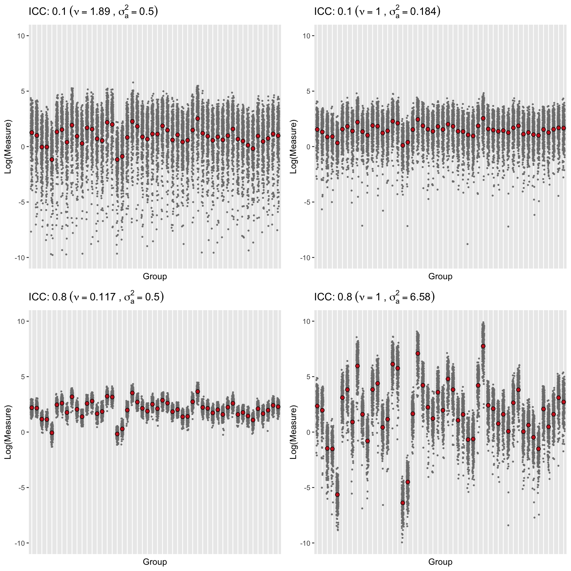
## 1: 0.1003386Finally, here are some plots of the generated observations and the group means on the log scale. The plots in each row have the same ICC but different underlying mean and dispersion parameters. I find these plots interesting because looking across the columns or up and down the two rows, they provide some insight to the interplay of group means and dispersion on the ICC …
Reference:
Nakagawa, Shinichi, Paul CD Johnson, and Holger Schielzeth. “The coefficient of determination R 2 and intra-class correlation coefficient from generalized linear mixed-effects models revisited and expanded.” Journal of the Royal Society Interface 14.134 (2017): 20170213.