A Bayesian implementation of a latent threshold model

The model

Before laying out the model (described in much more detail in the Stan User’s Guide), I should highlight two key features. First, we assume that the distribution of the outcome differs on either side of the threshold. In this example, we expect that the outcome data for antibody levels below the threshold are distributed as \(N(\alpha, \sigma)\), and that data above the threshold are \(N(\beta, \sigma)\). Second, since we do not know the threshold value, the likelihood is specified as a mixture across the range of all possible thresholds; the posterior distribution of the parameters \(\alpha\) and \(\beta\) reflect the uncertainty where the threshold lies.

The observed data include the continuous outcome \(\textbf{y}\) and a continuous antibody measure \(\textbf{x}\). There are \(M\) possible pre-specified thresholds that are reflected in the vector \(\mathbf{c}\). Each candidate threshold is treated as a discrete quantity and a probability \(\lambda_m\) is attached to each. Here is the model for the outcome conditional on the distribution parameters as well as the probability of the thresholds:

\[p(\textbf{y}|\alpha, \beta, \sigma, \mathbf{\lambda}) = \sum_{m=1}^M \lambda_m \left(\prod_{i: \; x_i < c[m]} \text{normal}(y_i | \alpha, \sigma) \prod_{i: \; x_i \ge c[m]} \text{normal}(y_i | \beta, \sigma)\right)\]

Implmentation in Stan

Here is a translation of the model into Stan. The data for the model include the antibody level \(x\), the outcome \(y\), and the candidate thresholds included in the vector \(\mathbf{c}\) which has length \(M\). In this example, the candidate vector is based on the range of observed antibody levels.

data {
  int<lower=1> N;                // number of observations
  real x[N];                     // antibody measures
  real y[N];                     // outcomes
    
  int<lower=1> M;                // number of candidate thresholds
  real c[M];                     // candidate thresholds
}

At the outset, equal probability will be assigned to each of the \(M\) candidate thresholds, which is \(1/M\). Since Stan operates in log-probabilities, this is translated to \(\text{log}(1/M) = \text{-log}(M)\):

transformed data {
  real lambda;
  lambda = -log(M);
}

The three parameters that define the two distributions (above and below the threshold) are \(\alpha\), \(\beta\), and \(\sigma\):

parameters {
  real alpha;
  real beta;
  real<lower=0> sigma;
}

This next block is really the implementation of the threshold model. \(\mathbf{lp}\) is a vector of log probabilities, where each element represents the log of each summand in the model specified above.

transformed parameters {
  vector[M] lp;
  lp = rep_vector(lambda, M);
  
  for (m in 1:M)
    for (n in 1:N)
      lp[m] = lp[m] + normal_lpdf(y[n] | x[n] < c[m] ? alpha : beta, sigma);
}

The notation y[n] | x[n] < c[m] ? alpha : beta, sigma is Stan’s shorthand for an if-then-else statement (this is note Stan code!):

if x[n] < c[m] then 
  y ~ N(alpha, sigma)
else if x[n] >= c[m] then
  y ~ N(beta, sigma)

And finally, here is the specification of the priors and the full likelihood, which is the sum of the log-likelihoods across the candidate thresholds. The function log_sum_exp executes the summation across the \(M\) candidate thresholds specified in the model above.

model {
  alpha ~ student_t(3, 0, 2.5);
  beta ~ student_t(3, 0, 2.5);
  sigma ~ exponential(1);
  
  target += log_sum_exp(lp);
}

Data generation

The data generated to explore this model is based on the same data definitions I used in the last post to explore the MLE model.

library(simstudy)
set.seed(87654)

d1 <- defData(varname = "antibody", formula = 0, variance = 1, dist = "normal")
d1 <- defData(d1, varname = "latent_status", formula = "-3 + 6 * (antibody > -0.7)",
              dist = "binary", link = "logit")
d1 <- defData(d1, varname = "y", formula = "0 + 3 * latent_status", 
              variance = 1, dist = "normal")

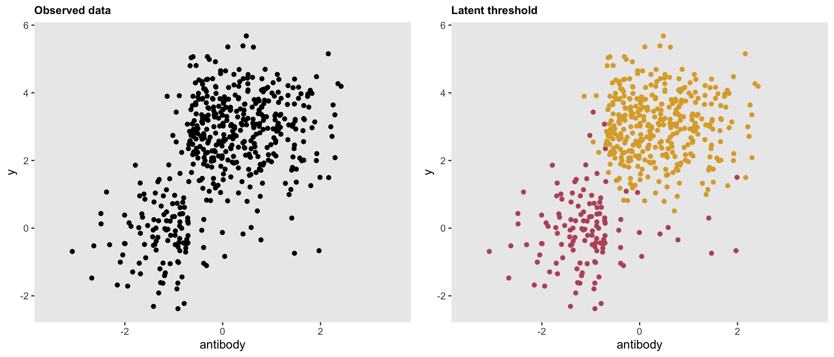
dd <- genData(500, d1)

The threshold is quite apparent here. In the right hand plot, the latent classes are revealed.

Model fitting

We use the rstan package to access Stan, passing along the observed antibody data, outcome data, as well as the candidate thresholds:

library(rstan)

rt <- stanc("/.../threshold.stan");
sm <- stan_model(stanc_ret = rt, verbose=FALSE)

N <- nrow(dd3)
y <- dd3[, y]
x <- dd3[, antibody] 
c <- seq(round(min(x), 1), round(max(x), 1), by = .1)
M <- length(c)

studydata3 <- list(N=N, x=x, y=y, M=M, c=c)
fit3 <-  sampling(sm, data = studydata3, iter = 3000, warmup = 500, 
                  cores = 4L, chains = 4, control = list(adapt_delta = 0.8))

The first order of business is to make sure that the MCMC algorithm sampled the parameter space in a well-behave manner. Everything looks good here:

library(bayesplot)

posterior <- as.array(fit3) 
lp <- log_posterior(fit3)
np <- nuts_params(fit3)

color_scheme_set("mix-brightblue-gray")

mcmc_trace(posterior, pars = c("alpha","beta", "sigma"), 
                facet_args = list(nrow = 3), np = np) + 
  xlab("Post-warmup iteration")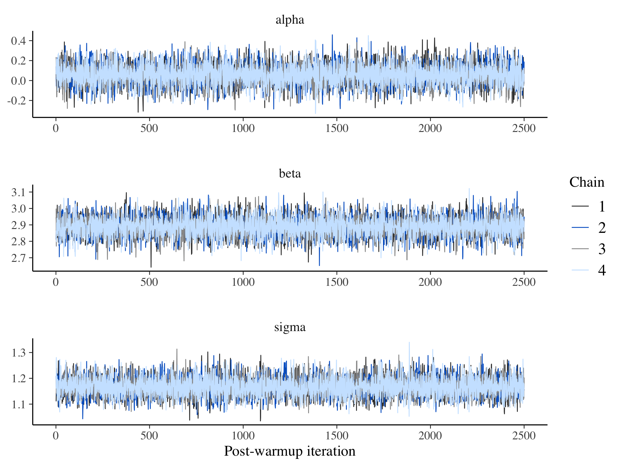

The posterior distributions of the three parameters of interest (\(\alpha\), \(\beta\), and \(\sigma\)) are quite close to the values used in the data generation process:

mcmc_intervals(posterior, pars = c("alpha","beta", "sigma"))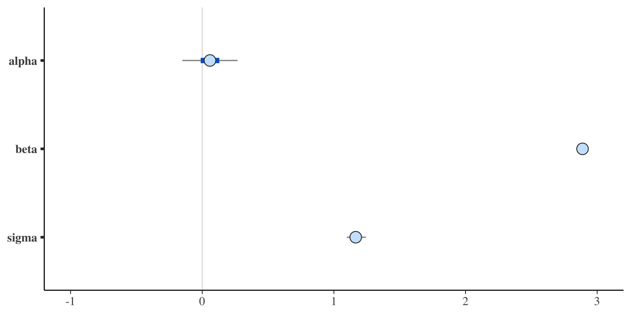

The posterior probability of the threshold

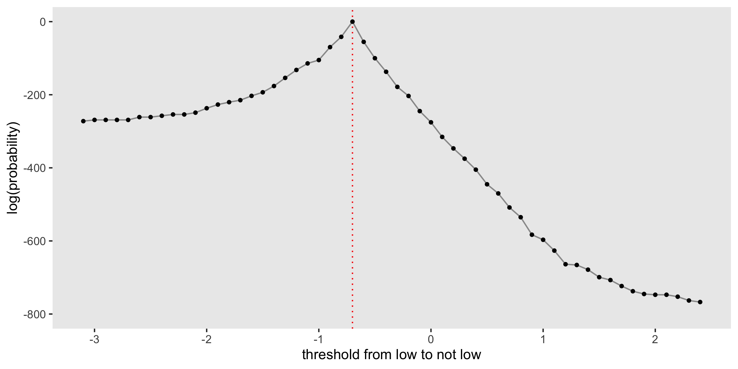
Even though the distributions of \(\alpha\), \(\beta\), and \(\sigma\) are marginal with respect to the candidate thresholds, we may still be interested in the posterior distribution of the thresholds. An approach to estimating this is described in the User’s Guide. I provide a little more detail and code for generating the plot in the addendum.

The plot shows the log-probability for each of the candidate thresholds considered, with a red dashed line drawn at \(-0.7\), the true threshold used in the data generation process. In this case, the probability (and log-probability) peaks at this point. In fact, there is a pretty steep drop-off on either side, indicating that we can have a lot of confidence that the threshold is indeed \(-0.7\).

When there is a single distribution

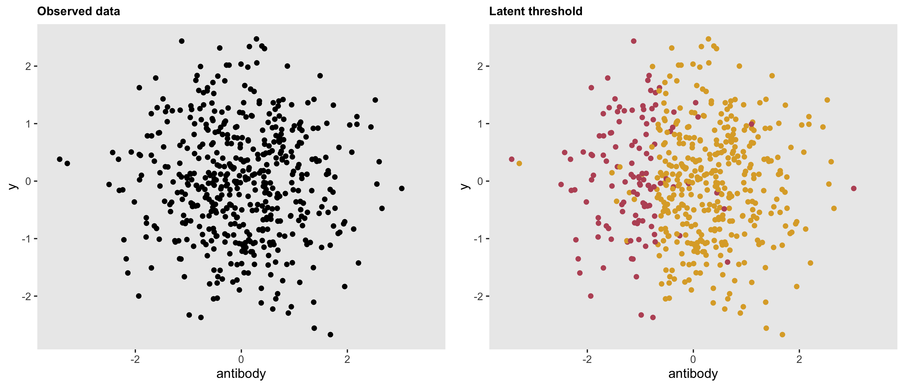
If we update the data definitions to generate a single distribution (i.e. the outcome is independent of the antibody measure), the threshold model with a struggles to identify a threshold, and the parameter estimates have more uncertainty.

d1 <- updateDef(d1, changevar = "y", newformula = "0")
dd <- genData(500, d1)

Here is a plot of the data based on the updated assumption:

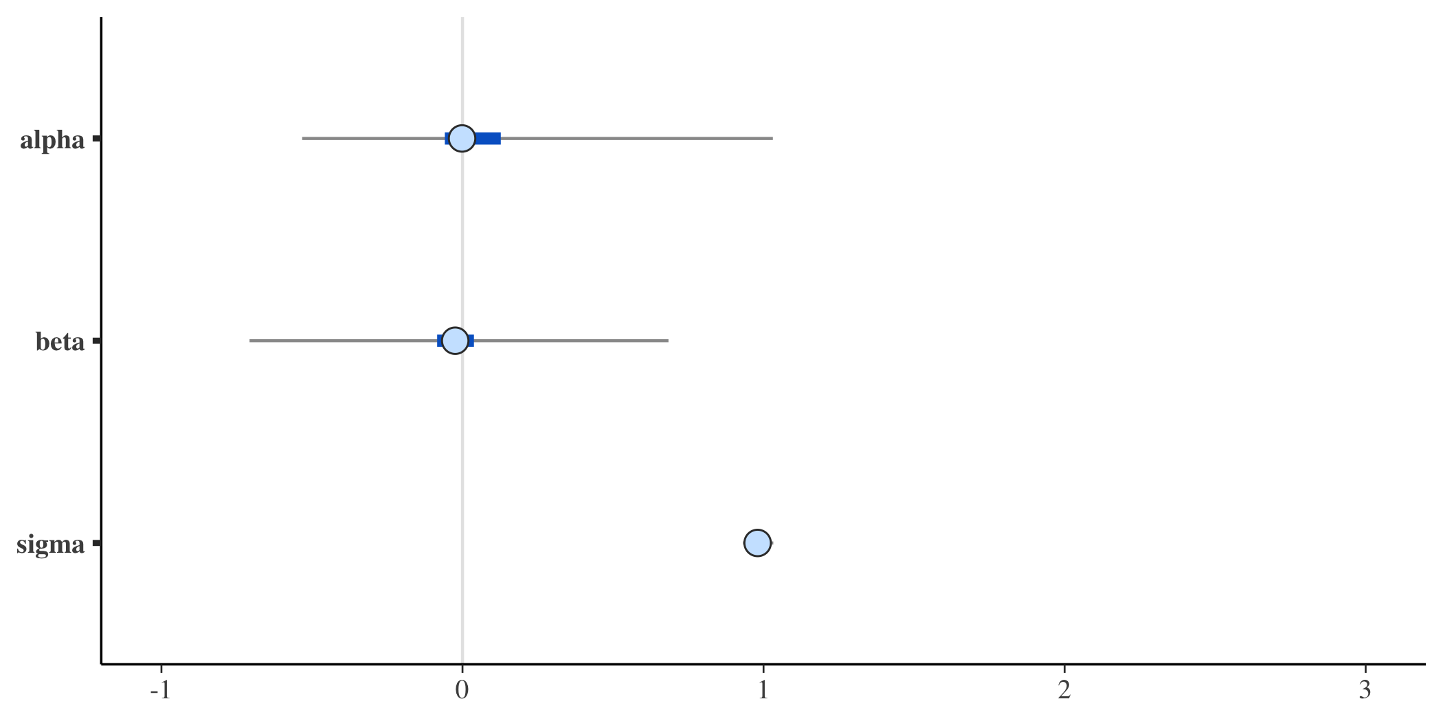
And here are the posterior probabilities for the parameters - now with much wider credible intervals:

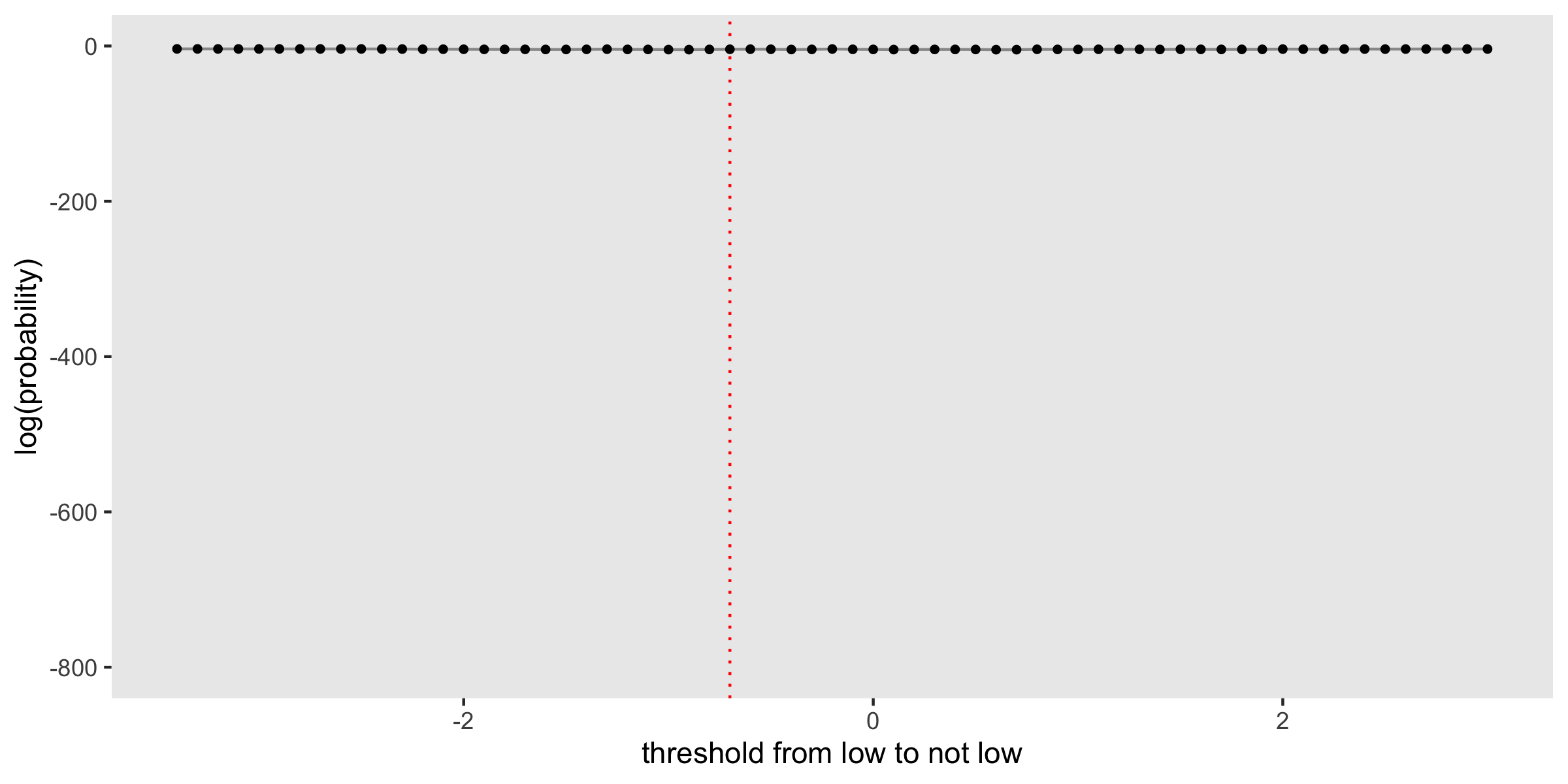
Here is the posterior distribution of thresholds, intentionally plotted to highlight the lack of distinction across the candidate thresholds:

Addendum - posterior probabilties of the threshold

Here’s a little more background on how the posterior probabilities for the threshold were calculated. As a reminder, \(\textbf{c}\) is a vector of candidate thresholds of length \(M\). We define a quantity \(q(c_m | data)\) as

\[ q(c_m | data) = \frac{1}{R}\sum_{r=1}^R \text{exp}(lp_{rc_m}) \] where \(lp_{cr_m}\) is the value of \(lp\) from the r’th draw for threshold candidate \(c_m\). We are actually interested in \(p(c_m|data\)), which is related to \(q\):

\[ p(c_m | data) = \frac{q(c_m | data)}{\sum_{m'=1}^M q(c_{m'}|data)} \]

The R code is a little bit involved, because the log-probabilities are so small that exponentiating them to recover the probabilities runs into floating point limitations. In the examples I have been using here, the log probabilities ranged from \(-4400\) to \(-700\). On my device the smallest value I can meaningfully exponentiate is \(-745\); anything smaller results in a value of 0, rendering it impossible to estimate \(q\).

To get around this problem, I used the mpfr function in the Rmfpr package. Here is a simple example to show how exponentiate a hihgly negative variable \(b\). A helper variable \(a\) is specified to set the precision, which can then be used to derive the desired result, which is \(\text{exp}(b)\).

Everything is fine if \(b \ge -745\):

library(Rmpfr)

b <- -745
exp(b)

## [1] 4.94e-324

For \(b<-745\), we have floating point issues:

b <- -746
exp(b)

## [1] 0

So, we turn to mpfr to get the desired result. First, specify \(a\) with the proper precision:

(a <- mpfr(exp(-100), precBits=64))

## 1 'mpfr' number of precision  64   bits 
## [1] 3.72007597602083612001e-44

And now we can calculate \(\text{exp}(b)\):

a^(-b/100)

## 1 'mpfr' number of precision  64   bits 
## [1] 1.03828480951583225515e-324

The code to calculate \(\text{log}(p_{c_m})\) extracts the draws of \(lp\) from the sample, exponentiates, and sums to get the desired result.

library(glue)

a <- mpfr(exp(-100), precBits=64)

qc <- NULL
for(m in 1:M) {
  lp.i <- glue("lp[{m}]")
  le <- rstan::extract(fit3, pars = lp.i)[[1]]
  q <- a^(-le/100)
  qc[m] <- sum(q)
}

qcs <- mpfr2array(qc, dim = M)
lps <- log(qcs/sum(qcs))
dps <- data.table(c, y=as.numeric(lps))

ggplot(data = dps, aes(x = c, y = y)) +
  geom_vline(xintercept = -0.7, color = "red", lty = 3) +
  geom_line(color = "grey60") +
  geom_point(size = 1) +
  theme(panel.grid = element_blank()) +
  ylab("log(probability)") +
  xlab("threshold from low to not low") +
  scale_y_continuous(limits = c(-800, 0))