In the previous post, I simulated data from a hypothetical RCT that had heterogeneous treatment effects across subgroups defined by three covariates. I presented two Bayesian models, a strongly pooled model and an unpooled version, that could be used to estimate all the subgroup effects in a single model. I compared the estimates to a set of linear regression models that were estimated for each subgroup separately.
My goal in doing these comparisons is to see how often we might draw the wrong conclusion about subgroup effects when we conduct these types of analyses. In a typical frequentist framework, the probability of making a mistake is usually considerably greater than the 5% error rate that we allow ourselves, because conducting multiple tests gives us more chances to make a mistake. By using Bayesian hierarchical models that share information across subgroups and more reasonably measure uncertainty, I wanted to see if we can reduce the chances of drawing the wrong conclusions.
Simulation framework
The simulations used here are based on the same general process I used to generate a single data set the last time around. The key difference is that I now want to understand the operating characteristics of the models, and this requires many data sets (and their model fits). Much of the modeling is similar to last time, so I’m primarily showing new code.
This is a pretty computing intensive exercise. While the models don’t take too long to fit, especially with only 150 observations per data set, fitting 2500 sets of models can take some time. As I do for all the simulations that require repeated Bayesian estimation, I executed all of this on a high-performance computer. I used a framework similar to what I’ve described for conducting power analyses and exploring the operating characteristics of Bayesian models.
Definitions
The definitions of the data generation process are the same as in the previous post, except I’ve made the generation of theta more flexible. Last time, I fixed the coefficients (\(\tau\)’s) at specific values. Here, the \(\tau\)’s can vary from iteration to iteration. Even though I am generating data with no treatment effect, I am taking a Bayesian point of view on this - so that the treatment effect parameters will have a distribution that is centered around 0 with very low variance.
library(cmdstanr)
library(simstudy)
library(posterior)
library(data.table)
library(slurmR)

setgrp <- function(a, b, c) {

  if (a==0 & b==0 & c==0) return(1)
  if (a==1 & b==0 & c==0) return(2)
  if (a==0 & b==1 & c==0) return(3)
  if (a==0 & b==0 & c==1) return(4)
  if (a==1 & b==1 & c==0) return(5)
  if (a==1 & b==0 & c==1) return(6)
  if (a==0 & b==1 & c==1) return(7)
  if (a==1 & b==1 & c==1) return(8)

}

s_define <- function() {

  d <- defData(varname = "a", formula = 0.6, dist="binary")
  d <- defData(d, varname = "b", formula = 0.4, dist="binary")
  d <- defData(d, varname = "c", formula = 0.3, dist="binary")
  d <- defData(d, varname = "theta",
    formula = "..tau[1] + ..tau[2]*a  + ..tau[3]*b + ..tau[4]*c +
               ..tau[5]*a*b + ..tau[6]*a*c + ..tau[7]*b*c + ..tau[8]*a*b*c",
    dist = "nonrandom"
  )

  drx <- defDataAdd(
    varname = "y", formula = "0 + theta*rx",
    variance = 16,
    dist = "normal"
  )

  return(list(d = d, drx = drx))

}
Data generation
We are generating the eight values of tau for each iteration from a \(N(\mu = 0, \sigma = 0.5)\) distribution before generating theta and the outcome y:
s_generate <- function(n, list_of_defs) {

  list2env(list_of_defs, envir = environment())

  tau <- rnorm(8, 0, .5)

  dd <- genData(n, d)
  dd <- trtAssign(dd, grpName = "rx")
  dd <- addColumns(drx, dd)

  dd[, grp := setgrp(a, b, c), keyby = id]

  dd[]

}
Looking at a single data set, we can see that theta is close to, but is not exactly 0, as we would typically do in simulation using a frequentist framework (where the parameters are presumed known).
set.seed(298372)

defs <- s_define()
s_generate(10, defs)
## id a b c theta rx y grp
## 1: 1 0 0 1 0.34 0 -3.45 4
## 2: 2 1 0 1 0.78 1 3.20 6
## 3: 3 0 0 0 -0.28 1 7.29 1
## 4: 4 0 1 0 -0.37 1 2.76 3
## 5: 5 0 0 0 -0.28 0 -0.48 1
## 6: 6 1 0 0 -0.25 0 1.09 2
## 7: 7 0 0 0 -0.28 0 -1.45 1
## 8: 8 0 0 1 0.34 1 -5.78 4
## 9: 9 1 0 0 -0.25 1 2.97 2
## 10: 10 1 0 0 -0.25 0 -1.25 2Model fitting
The models here are precisely how I defined it in the last post. The code is a bit involved, so I’m not including it - let me know if you’d like to see it. For each data set, I fit a set of subgroup-specific linear regression models (as well as an overall model that ignored the subgroups), in addition to the two Bayesian models described in the previous post. Each replication defines the data, generates a new data set, and estimates the three different models before returning the results.
s_model <- function(dd, mod_pool, mod_nopool) {
  ...
}

s_replicate <- function(x, n, mod_pool, mod_nopool) {

  set_cmdstan_path(path = "/.../cmdstan/2.25.0")

  defs <- s_define()
  generated_data <- s_generate(n, defs)
  estimates <- s_model(generated_data, mod_pool, mod_nopool)

  estimates[]
}
The computation is split up so that 50 multi-core computing nodes run 50 replications. There’s actually parallelization in parallel, as each of the nodes has multiple processors so the Bayesian models can be estimated with parallel chains:
set_cmdstan_path(path = "/gpfs/share/apps/cmdstan/2.25.0")

model_pool <- cmdstan_model("/.../subs_pool_hpc.stan")
model_nopool <- cmdstan_model("/.../subs_nopool_hpc.stan")

job <- Slurm_lapply(
  X = 1:2500,
  FUN = s_replicate,
  n = 150,
  mod_pool = model_pool,
  mod_nopool = model_nopool,
  njobs = 50,
  mc.cores = 4L,
  job_name = "i_subs",
  tmp_path = "/.../scratch",
  plan = "wait",
  sbatch_opt = list(time = "12:00:00", partition = "cpu_short", `mem-per-cpu` = "5G"),
  export = c("s_define", "s_generate", "s_model"),
  overwrite = TRUE
)

job
res <- Slurm_collect(job)

save(res, file = "/.../sub_0.rda")
Results
The figure shows the results from 80 models. Each column is a different subgroup (and the last is the overall treatment effect estimate). The intervals are the 95% credible intervals from the Bayesian models, and the 95% confidence interval from the linear regression model. The intervals are color coded based on whether the interval includes 0 (grey) or not (red). The red intervals are cases where we might incorrectly conclude that there is indeed some sort of effect. There are many more red lines for the linear regression estimates compared to either of the Bayesian models:
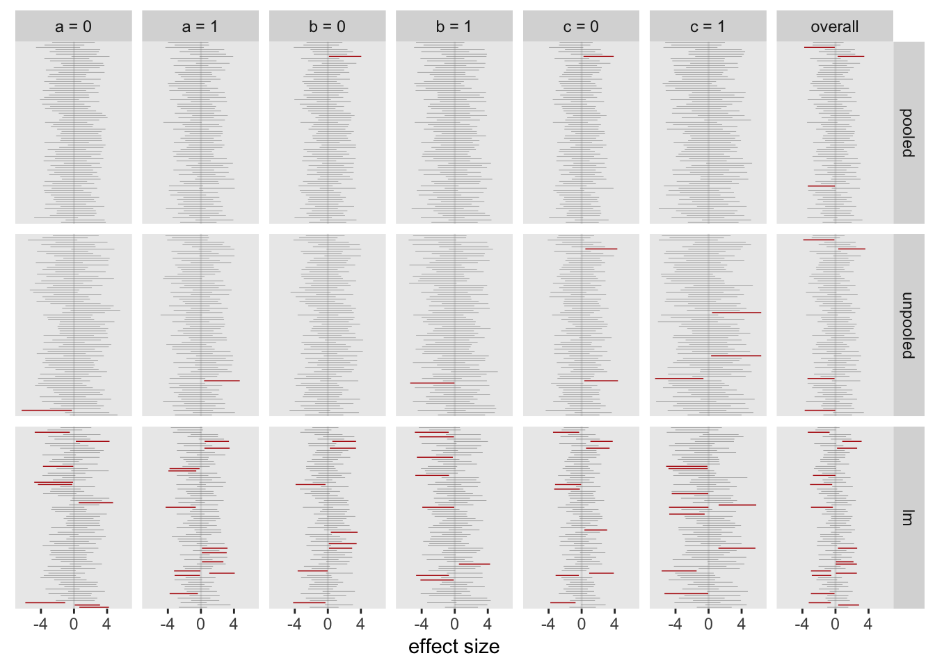
For the full set of 2500 replications, about 5% of the intervals from the pooled Bayes did not include 0, lower than the unpooled model, and far below the approach using individual subgroup regression models:
##    pooled unpooled   lm
## 1:  0.051     0.11 0.37
I started off the last post by motivating this set of simulations with an experience I recently had with journal reviewers who were skeptical of an analysis of a subgroup effect size. I’m not sure that the journal reviewers would buy the approach suggested here, but it seems that pooling estimates across subgroups provides a viable way to guard against making overly strong statements about effect sizes when they are not really justified.