Sample size determination in the context of Bayesian analysis

Bayesian inference

In the Bayesian framework, all statistical inference is based on the estimated posterior probability distribution for the parameter(s) of interest (say \(\theta\)) once we have observed the data: \(P(\theta | \text{data})\). In addition to extracting the mean or median of the distribution as a point estimate, we can get a measure of uncertainty by extracting quantiles from the distribution (a 95% interval comes to mind, though there is no reason to be limited by that convention).

Alternatively, we can make a probability statement about the parameter being above or below a threshold of effectiveness. For example if we are estimating a log-odds ratio for an intervention that prevents a bad outcome, we might be interested in \(P(log(OR) < 0).\) We may even pre-specify that the trial will be considered a success if \(P(log(OR) < 0) > 0.95.\)

library(simstudy)
library(data.table)
library(ggplot2)
library(cmdstanr)
library(posterior)
library(bayesplot)

Data generation

To investigate, I will use a simple binary outcome \(Y\) that is changed by exposure or intervention \(A\). In this first case, I will randomly select a log-odds ratio from \(N(\mu = -1, \sigma = 0.5).\)

defB <- defDataAdd(varname = "Y", formula = "-2 + ..lor * A", 
  dist = "binary", link="logit")

set.seed(21)
lor <- rnorm(1, -1, 0.5)

dT <- genData(200)
dT <- trtAssign(dT, grpName = "A")
dT <- addColumns(defB, dT)

Model fitting

I am primarily interested in recovering the log-odds ratio use to generate the data using a simple Bayesian model, written here in Stan. The parameter of interest in the Stan model is \(\beta\), log-odds ratio. The prior distribution is \(t_{student}(df=3, \mu=0, \sigma=5).\)

data {
  int<lower=0> N;
  int<lower=0,upper=1> y[N];
  vector[N] x;
  real mu;
  real s;
}

parameters {
  real alpha;
  real beta;
}

model {
  beta ~ student_t(3, mu, s);
  y ~ bernoulli_logit(alpha + beta * x);
}

To estimate the posterior distribution, I am using the R package cmdstanr:

mod <- cmdstan_model("code/bayes_logistic.stan")

fit <- mod$sample(
  data =  list(N=nrow(dT), y=dT$Y, x=dT$A, mu=0, s=5),
  refresh = 0,
  chains = 4L,
  parallel_chains = 4L,
  iter_warmup = 1000,
  iter_sampling = 4000,
  step_size = 0.1,
  show_messages = FALSE
)

## Running MCMC with 4 parallel chains...
## 
## Chain 1 finished in 0.2 seconds.
## Chain 2 finished in 0.2 seconds.
## Chain 3 finished in 0.2 seconds.
## Chain 4 finished in 0.2 seconds.
## 
## All 4 chains finished successfully.
## Mean chain execution time: 0.2 seconds.
## Total execution time: 0.4 seconds.

(If you’re impressed at how fast that model ran, it is because it is on my new MacBook Pro with the new Apple M1 chip - 4 or 5 times faster than my previous MacBook Pro with an Intel chip. It took me a while to get R, RStudio, and particularly, cmdstan up and running, but once I did, it has been totally worth it.)

First thing to check, of course, is whether the sampling from the posterior distribution was well-behaved. Here is a trace plot for the parameter \(\beta\):

draws_array <- as_draws_array(fit$draws())
mcmc_trace(draws_array, pars = "beta")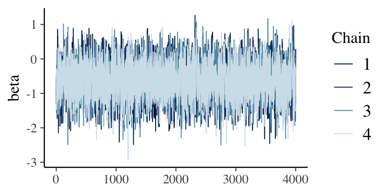

Here are the summary statistics of the posterior distribution. Based on these data, the median log-odds ratio is \(-0.61\) and \(P(lor < 0) = 89\%\):

res <- data.table(fit$summary(variables = "beta"))[, 
          .(median, sd, q95, len = q95-q5)]

betas <- data.table(beta = as.matrix(draws_array[,,"beta"]))
res$p0 <- mean(betas$beta.V1 < 0)

res

##        median       sd       q95      len      p0
## 1: -0.6050845 0.511862 0.2103548 1.673138 0.88875

A plot of the posterior distribution is the best way to fully assess the state of knowledge about the parameter having observed this data set. The density plot includes a vertical dashed line at the median, and the dark shading indicates lowest \(95\%\) of the density. The fact that the cutoff point \(0\) lies within the bottom \(95\%\) makes it clear that the threshold was not met.

d <- density(draws_array[,,"beta"], n = 1024)
plot_points <- as.data.table(d[c("x", "y")])
median_xy <- plot_points[findInterval(res$median, plot_points$x)]

ggplot(data = plot_points, aes(x = x, y = y)) +
  geom_area(aes(fill = (x < res$q95))) +
  geom_segment(x = median_xy$x, xend=median_xy$x, y=0, yend = median_xy$y,
               size = 0.2, color = "white", lty=3) +
  scale_fill_manual(values = c("#adc3f2", "#5886e5")) +
  theme(panel.grid = element_blank(),
        legend.position = "none")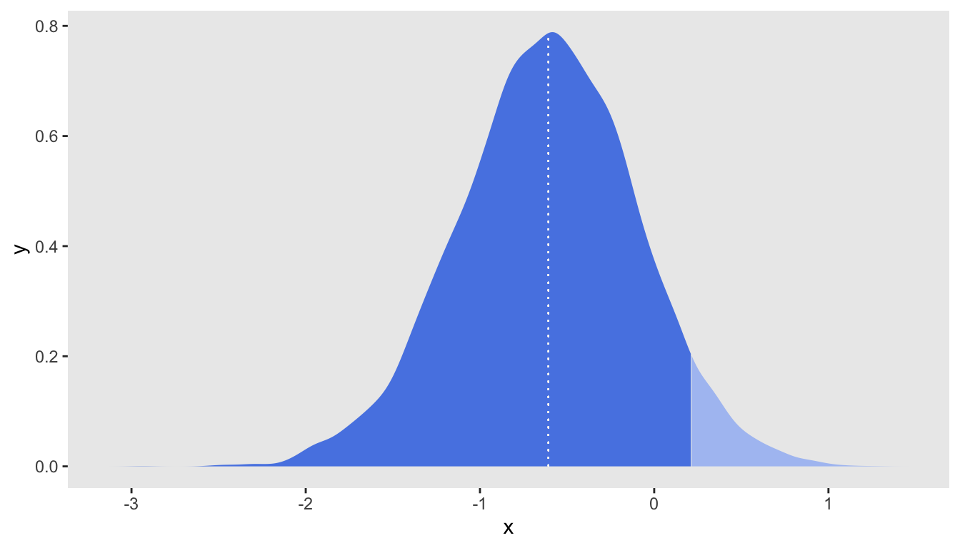

Bayesian power

If we want to assess what kind of sample sizes we might want to target in study based on this relatively simple design (binary outcome, two-armed trial), we can conduct a Bayesian power analysis that has a somewhat different flavor from the more typical frequentist Bayesian that I typically do with simulation. There are a few resources I’ve found very useful here: this book by Spiegelhalter et al and these two papers, one by Wang & Gelfand and another by De Santis & Gubbiotti

When I conduct a power analysis within a frequentist framework, I usually assume set of fixed/known effect sizes, and the hypothesis tests are centered around the frequentist p-value at a specified level of \(\alpha\). The Bayesian power analysis differs with respect to these two key elements: a distribution of effect sizes replaces the single fixed effect size to accommodate uncertainty, and the posterior distribution probability threshold (or another criteria such as the variance of the posterior distribution or the length of the 95% credible interval) replaces the frequentist hypothesis test.

We have a prior distribution of effect sizes. De Santis and Gubbiotti suggest it is not necessary (and perhaps less desirable) to use the same prior used in the model fitting. That means you could use a skeptical (conservative) prior centered around 0, in the analysis, but use a prior for data generation that is consistent with a clinically meaningful effect size. In the example above the analysis prior was

\[ \beta \sim t_{student}(df = 3, \mu = 0, \sigma = 5) \]

and the data generation prior was

\[ \beta \sim N(\mu = -1, \sigma = 0.5).\]

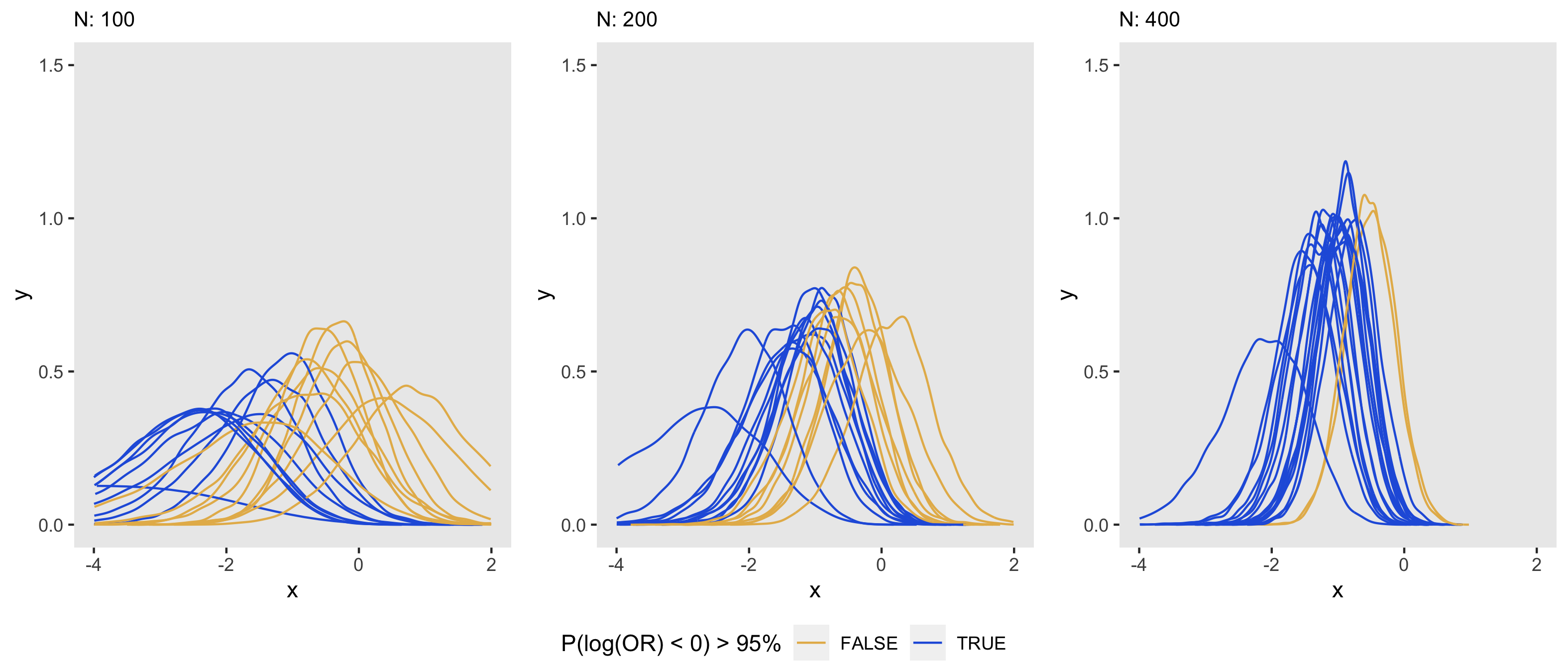
To conduct the Bayesian power analysis, I replicated the simulation and model fitting shown above 1000 times for each of seven different sample sizes ranging from 100 to 400. (Even though my laptop is quite speedy, I used the NYU Langone Health high performance cluster Big Purple to do this, because I wanted to save a few hours.) I’m not showing the parallelized code in this post, but take a look here for an example similar to this. (I’m happy to share with anyone if you’d like to have the code. Updated 7/1/2021: code has been added in the Addendum below.)

The plots below show a sample of 20 posterior distributions taken from the 1000 generated for each of three sample sizes. As in the frequentist context, an increase in sample size appears to reduce the variance of the posterior distribution estimated in a Bayesian model. We can see visually that as the sample size increases, the distribution collapses towards the mean or median, which has a direct impact on how confident we are in drawing conclusions from the data; in this case, it is apparent that as sample size increases, the proportion of posterior distributions meet the 95% threshold increases.

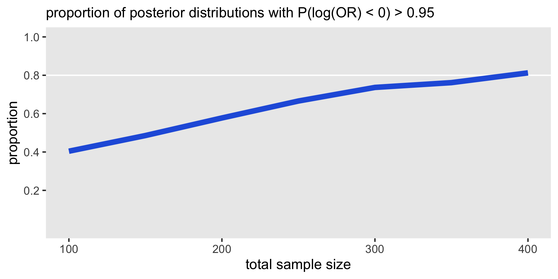
Here is a curve that summarizes the probability of a posterior distribution meeting the 95% threshold at each sample size level. At a size of 400, 80% of the posterior distributions (which are themselves based on data generated from varying effect sizes specified by the data generation prior and the analysis prior) would lead us to conclude that the trial is success.

Addendum

Here is the full R code for the Bayesian power analysis using simulation. I am including the slurmR code that I used to execute on the HPC:

library(simstudy)
library(data.table)
library(ggplot2)
library(bayesplot)
library(posterior)
library(cmdstanr)
library(slurmR)
library(collapse)

s_define <- function() {
    
  defB <- defDataAdd(varname = "Y", formula = "-2 + ..lor * rx", 
                     dist = "binary", link="logit")
  
  return(list(defB = defB)) # list_of_defs is a list of simstudy data definitions
}

s_generate <- function(list_of_defs, argsvec) {
    
  list2env(list_of_defs, envir = environment())
  list2env(as.list(argsvec), envir = environment())
  
  #--- add data generation code ---#
  
  lor <- rnorm(1, mu.lor, sigma.lor)
  
  dT <- genData(nobs)
  dT <- trtAssign(dT, grpName = "rx")
  dT <- addColumns(defB, dT)
  
  return(dT[])
  
}

s_model <- function(generated_data, mod, argsvec) {
    
  list2env(as.list(argsvec), envir = environment())
    
  dt_to_list <- function(dx) {
    
    N <- nrow(dx)                  ## number of observations 
    y <- dx$Y                      ## individual outcome 
    x <- dx$rx                     ## treatment arm for individual 
    s <- t_sigma
    mu <- 0 # can be mu.lor
      
    list(N=N, y=y, x=x, s=s, mu = mu)
  }

  fit <- mod$sample(
    data = dt_to_list(generated_data),
    refresh = 0,
    chains = 4L,
    parallel_chains = 4L,
    iter_warmup = 1000,
    iter_sampling = 4000,
    step_size = 0.1,
    show_messages = FALSE
  )
    
  res <- data.table(fit$summary(variables = "beta"))[, .(median, sd, q95, len = q95-q5)]
    
  draws_array <- as_draws_array(fit$draws())
  betas <- data.table(beta = as.matrix(draws_array[,,"beta"]))
  res$p0 <- mean(betas$beta.V1 < 0)

  return(res) # model_results is a data.table
  }

s_single_rep <- function(list_of_defs, argsvec, mod) {
    
  set_cmdstan_path(path = "/gpfs/share/apps/cmdstan/2.25.0")
  
  list_of_defs <- s_define()
  generated_data <- s_generate(list_of_defs, argsvec)
  model_results <- s_model(generated_data, mod, argsvec)
  
  return(model_results)
}
  
s_replicate <- function(argsvec, nsim, mod) {
  
  list_of_defs <- s_define()
  
  model_results <- 
    lapply(
      X = 1 : nsim, 
      FUN = function(x) s_single_rep(list_of_defs, argsvec, mod)
    )
  
  #--- add summary statistics code ---#
  
  model_sums <- unlist2d(lapply(model_results, function(x) x), 
    idcols = "replicate", DT = TRUE)
  
  summary_stats <- model_sums[ , 
    .(p_95 = mean(p0 >= 0.95), 
      p_len = mean(len <= 2),
      p_sd = mean(sd <= 0.5))
  ]
  
  model_ests <- data.table(t(argsvec), summary_stats)

  return(model_ests)
  
}

###

scenario_list <- function(...) {
  argmat <- expand.grid(...)
  return(asplit(argmat, MARGIN = 1))
}

mu.lor <- c(0, -0.5, -1.0, -1.5)
sigma.lor <- c(0.25)
nobs <- c(100, 150, 200, 250, 300, 350, 400)
t_sigma <- c(1, 5, 10)

scenarios <- scenario_list(mu.lor = mu.lor, sigma.lor = sigma.lor, 
                           nobs = nobs, t_sigma = t_sigma)

set_cmdstan_path(path = ".../cmdstan/2.25.0")
mod <- cmdstan_model("present.stan")

job <- Slurm_lapply(
  X = scenarios, 
  FUN = s_replicate, 
  mod = mod,
  nsim = 1200,
  njobs = min(length(scenarios), 90L), 
  mc.cores = 4L,
  job_name = "i_bp",
  tmp_path = "/gpfs/data/troxellab/ksg/scratch",
  plan = "wait",
  sbatch_opt = list(time = "03:00:00", partition = "cpu_short"),
  export = c("s_single_rep", "s_define", "s_generate", "s_model"),
  overwrite = TRUE
)

summary_stats <- Slurm_collect(job)
final_tab <- rbindlist(summary_stats)

save(final_tab, file = ".../bp.rda")

References:

Wang, Fei, and Alan E. Gelfand. “A simulation-based approach to Bayesian sample size determination for performance under a given model and for separating models.” Statistical Science 17, no. 2 (2002): 193-208.
Spiegelhalter, David J., Keith R. Abrams, and Jonathan P. Myles. Bayesian approaches to clinical trials and health-care evaluation. Vol. 13. John Wiley & Sons, 2004.
De Santis, Fulvio, and Stefania Gubbiotti. “Sample Size Requirements for Calibrated Approximate Credible Intervals for Proportions in Clinical Trials.” International Journal of Environmental Research and Public Health 18, no. 2 (2021): 595.