Finding answers faster for COVID-19: an application of Bayesian predictive probabilities

Determining success

In this example, the outcome is the WHO 11-point ordinal scale for clinical status at 14 days, which ranges from 0 (uninfected and out of the hospital) to 10 (dead), with various stages of severity in between. As in COMPILE, I’ll use a Bayesian proportional odds model to assess the effectiveness of CP. The measure of effectiveness is an odds ratio (OR) that compares the cumulative odds of having a worse outcome for the treated group compared to the cumulative odds for the control group:

\[ \text{Cumulative odds for level } k \text{ in treatment arm } j =\frac{P(Y_{ij} \ge k)}{P(Y_{ij} \lt k)}, \ k \in \{1,\dots, 10\} \]

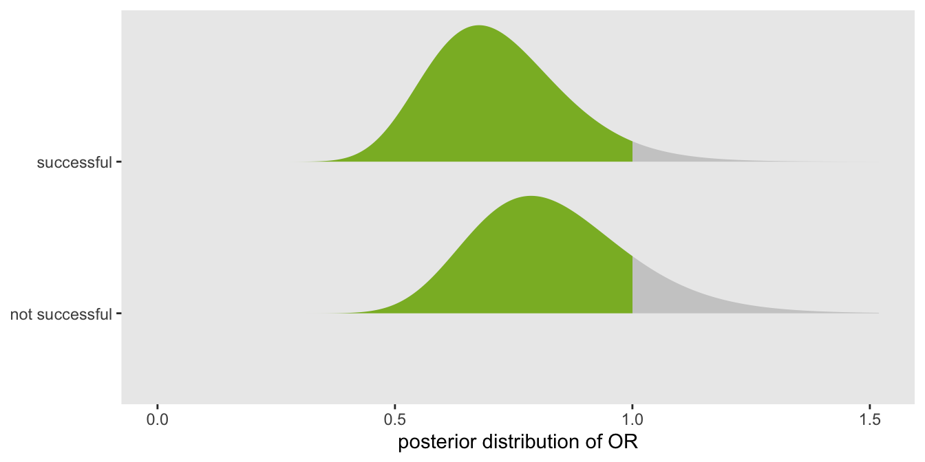
The goal is to reduce the odds of having a bad outcome, so a successful therapy is one where \(OR \lt 1\). In a Bayesian context, we estimate the posterior probability distribution of the \(OR\) (based on prior assumptions before we have collected any data). We will recommend the therapy in the case that most of the probability density lies to the left of 1; in particular we will claim success only when \(P(OR \lt 1) > 0.95\). For example, in the figure the posterior distribution on top would lead us to consider the therapy successful since 95% of the density falls below 1, whereas the distribution on the bottom would not:

Data set

This data set here is considerably simpler than the COMPILE data that has motivated all of this. Rather than structuring this example as a multi-study data set, I am assuming a rather simple two-arm design without any sort of clustering. I am including two binary covariates related to sex and age. The treatment in this case reduces the odds of worse outcomes (or increases the odds of better outcomes). For more detailed discussion of generating ordinal outcomes, see this earlier post (but note that I have flipped direction of cumulative probability in the odds formula).

library(simstudy)
library(data.table)

def1 <- defDataAdd(varname="male", formula="0.7", dist = "binary")
def1 <- defDataAdd(def1, varname="over69", formula="0.6", dist = "binary")
def1 <- defDataAdd(def1, 
  varname="z", formula="0.2*male + 0.3*over69 - 0.3*rx", dist = "nonrandom")

baseprobs <-  c(0.10, 0.15, 0.08, 0.07, 0.08, 0.08, 0.11, 0.10, 0.09, 0.08, 0.06)

RNGkind("L'Ecuyer-CMRG")
set.seed(9121173)

dd <- genData(450)
dd <- trtAssign(dd, nTrt = 2, grpName = "rx")
dd <- addColumns(def1, dd)
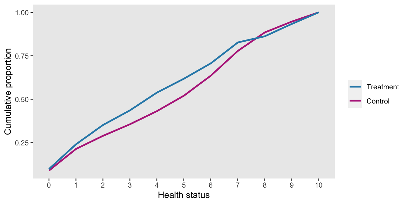
dd <- genOrdCat(dd, adjVar = "z", baseprobs = baseprobs, catVar = "y")

Here is a plot of the cumulative proportions by treatment arm for the first 450 patients in the (simulated) trial. The treatment arm has more patients with lower WHO-11 scores, so for the most part lies above the control arm line. (This may be a little counter-intuitive, so it may be worthwhile to think about it for a moment.)

Estimate a Bayes ordinal cumulative model

With the data from 450 patients in hand, the first step is to estimate a Bayesian proportional odds model, which I am doing in Stan. I use the package cmdstanr to interface between R and Stan.

Here is the model:

\[ \text{logit}\left(P(y_{i}) \ge k \right) = \tau_k + \beta_1 I(\text{male}) + \beta_2 I(\text{over69}) + \delta T_i, \ \ \ k \in \{ 1,\dots,10 \} \]

where \(T_i\) is the treatment indicator for patient \(i\), and \(T_i = 1\) when patient \(i\) receives CP. \(\delta\) represents the log odds ratio, so \(OR = e^{\delta}\). I’ve included the Stan code for the model in the the first addendum.

library(cmdstanr)

dt_to_list <- function(dx) {
  
  N <- nrow(dx)                               ## number of observations 
  L <- dx[, length(unique(y))]                ## number of levels of outcome 
  y <- as.numeric(dx$y)                       ## individual outcome 
  rx <- dx$rx                                 ## treatment arm for individual 
  x <- model.matrix(y ~ factor(male) + factor(over69), data = dx)[, -1]
  D <- ncol(x)
  
  list(N=N, L=L, y=y, rx=rx, x=x, D=D)
}

mod <- cmdstan_model("pprob.stan")

fit <- mod$sample(
  data = dt_to_list(dd),
  seed = 271263,
  refresh = 0,
  chains = 4L,
  parallel_chains = 4L,
  iter_warmup = 2000,
  iter_sampling = 2500,
  step_size = 0.1
)

## Running MCMC with 4 parallel chains...
## 
## Chain 4 finished in 56.9 seconds.
## Chain 1 finished in 57.8 seconds.
## Chain 3 finished in 58.0 seconds.
## Chain 2 finished in 60.7 seconds.
## 
## All 4 chains finished successfully.
## Mean chain execution time: 58.3 seconds.
## Total execution time: 61.0 seconds.

Extract posterior distribution

Once the model is fit, our primary interest is whether we can make a recommendation about the therapy. A quick check to verify if \(P(OR < 1) > 0.95\) confirms that we are not there yet.

library(posterior)

draws_df <- as_draws_df(fit$draws())
draws_dt <- data.table(draws_df[-grep("^yhat", colnames(draws_df))])

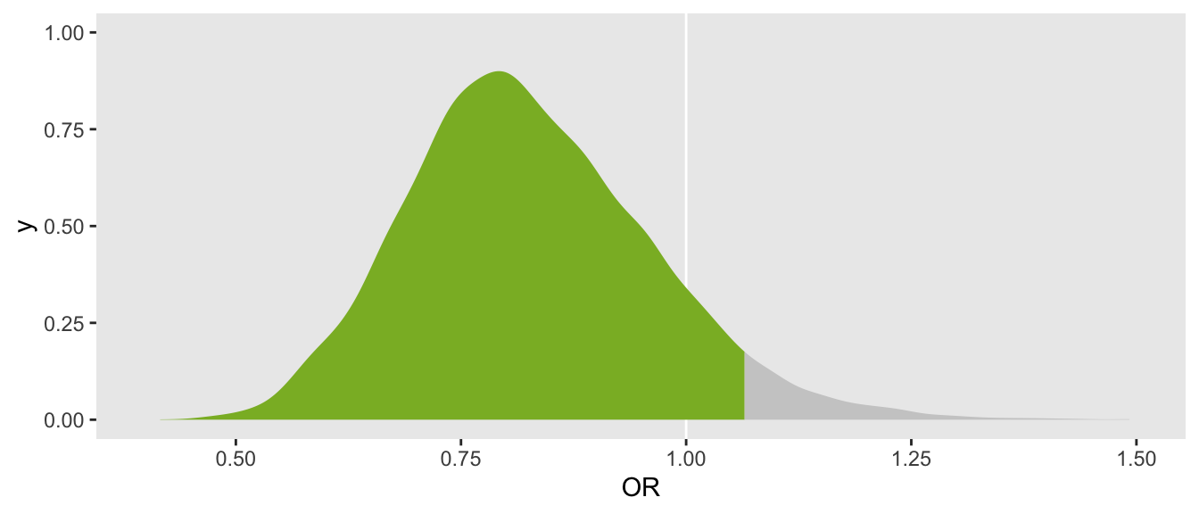
mean(draws_dt[, OR < 1])

## [1] 0.89

A plot that shows the bottom 95% portion of the density in blue makes it clear that the threshold has not been met:

The elements of the predictive probability

We have collected complete data from 450 patients out of an expect 500, though we are not yet ready declare success. An interesting question to ask at this point is “given what we have observed up until this point, what is the probability that we will declare success after 50 additional patients are included in the analysis?” If the probability is sufficiently high, we may decide to delay releasing the inconclusive results pending the updated data set. (On the other hand, if the probability is quite low, there may be no point in delaying.)

The prediction incorporates three potential sources of uncertainty. First, there is the uncertainty regarding the parameters, which is described by the posterior distribution. Second, even if we knew the parameters with certainty, the outcome remains stochastic (i.e. not pre-determined conditional on the parameters). Finally, we don’t necessarily know the characteristics of the remaining patients (though we may have some or all of that information if recruitment has been finished but complete follow-up has not).

In the algorithm that follows - the steps follow from these three elements of uncertainty:

1. Generate 50 new patients by bootstrap sampling (with replacement) from the observed patients. The distribution of covariates of the new 50 patients will be based on the original 450 patients.
2. Make a single draw from the posterior distribution of our estimates to generate a set of parameters.
3. Using the combination of new patients and parameters, generate ordinal outcomes for each of the 50 patients.
4. Combine this new data set with the 450 existing patients to create a single analytic file.
5. Fit a new Bayesian model with the 500-patient data set.
6. Record \(P(OR < 1)\) based on this new posterior distribution. If \(P(OR < 1)\) is \(\gt 95\%\), we consider the result to be a “success”, otherwise it is “not a success”.

We repeat this cycle, say 1000 times. The proportion of cycles that are counted as a success represents the predictive probability of success.

library(glue)

dd_new <- dd[, .(id = sample(id, 25, replace = TRUE)), keyby = rx]
dd_new <- merge(dd[, .(id, male, over69)], dd_new, by = "id")
dd_new[, id:= (nrow(dd) + 1):(nrow(dd) +.N)]

draw <- as.data.frame(draws_dt[sample(.N, 1)])

D <- dt_to_list(dd)$D
beta <- as.vector(x = draw[, glue("beta[{1:D}]")], mode = "numeric")
delta <- draw$delta
coefs <- as.matrix(c(beta, delta))

coefs

##       [,1]
## [1,]  0.22
## [2,]  0.60
## [3,] -0.19

tau <- as.vector(draw[grep("^tau", colnames(draw))], mode = "numeric")
tau <- c(tau, Inf)
cprop <- plogis(tau)
xprop <- diff(cprop)
baseline <- c(cprop[1], xprop) 

baseline

##  [1] 0.117 0.136 0.123 0.076 0.089 0.101 0.114 0.102 0.054 0.040 0.048

zmat <- model.matrix(~male + over69 + rx, data = dd_new)[, -1]
dd_new$z <- zmat %*% coefs
setkey(dd_new, id)

dd_new <- genOrdCat(dd_new, adjVar = "z", baseline, catVar = "y")

dx <- rbind(dd, dd_new)

fit_pp <- mod$sample(
  data = dt_to_list(dx),
  seed = 737163,
  refresh = 0,
  chains = 4L,
  parallel_chains = 4L,
  iter_warmup = 2000,
  iter_sampling = 2500,
  step_size = 0.1
)

## Running MCMC with 4 parallel chains...
## 
## Chain 2 finished in 79.4 seconds.
## Chain 4 finished in 79.7 seconds.
## Chain 3 finished in 80.1 seconds.
## Chain 1 finished in 80.5 seconds.
## 
## All 4 chains finished successfully.
## Mean chain execution time: 79.9 seconds.
## Total execution time: 80.6 seconds.

draws_pp <- data.table(as_draws_df(fit_pp$draws()))
draws_pp[, mean(OR < 1)]

## [1] 0.79

Estimating the predictive probability

The next step is to pull all these elements together in a single function that we can call repeatedly to estimate the predictive probability of success. This probability is estimated by calculating the proportion of iterations that result in a success.

Computing resources required for this estimation might be quite substantial. If we iterate 1000 times, we need to fit that many Bayesian models. And 1000 Bayesian model estimates could be prohibitive - a high performance computing cluster (HPC) may be necessary. (I touched on this earlier when I describe exploring the characteristic properties of Bayesian models.) I have provided the code below in the second addendum in case any readers are interested in trying to implement on an HPC.

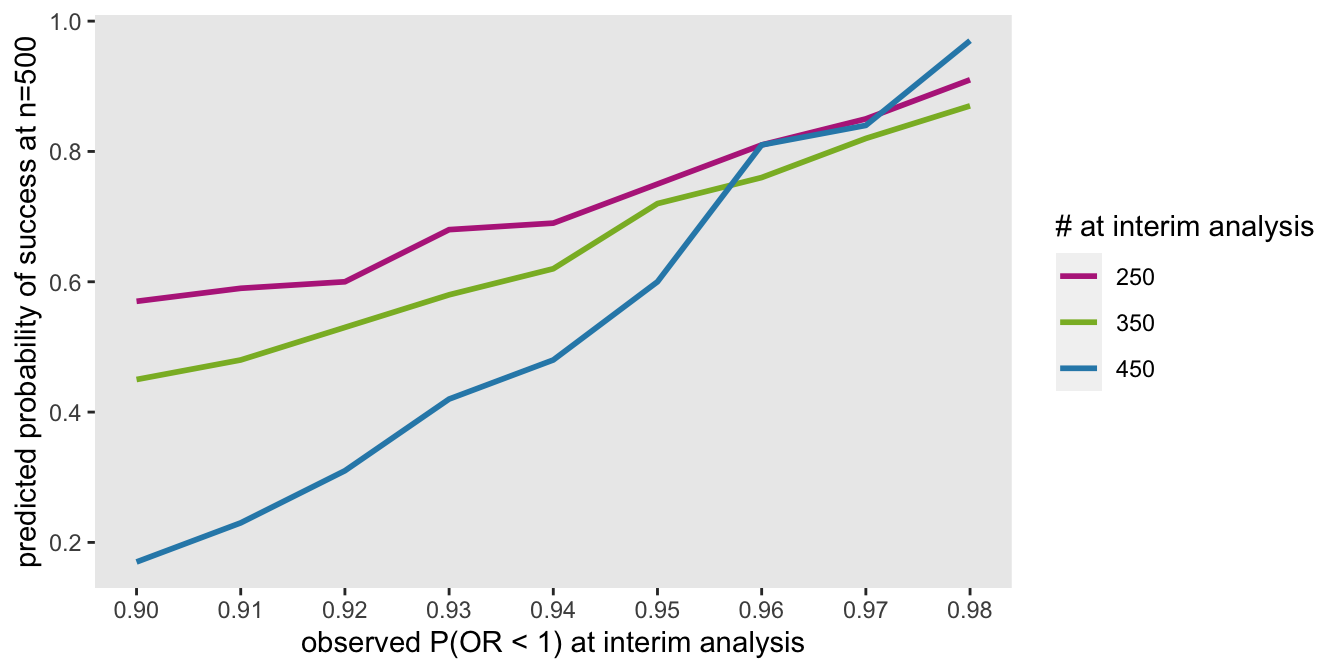
I’ll conclude with a figure that shows how predictive probabilities can vary depending on the observed sample size and \(P(OR < 1)\) for the interim data set. Based on the data generating process I’ve used here, if we observe a \(P(OR < 1) = 90\%\) at an interim look after 250 patients, it is considerably more probable that we will end up over 95% than if we observe that same probability at an interim look after 450 patients. This makes sense, of course, since the estimate at 450 patients will have less uncertainty, and adding 50 patients will not likely change to results dramatically. The converse is true after 250 patients.

Ultimately, the interpretation of the predictive probability will depend on the urgency of making a recommendation, the costs of waiting, the costs of deciding to soon, and other factors specific to the trial and those making the decisions.

Addendum A: stan code

data {
  int<lower=0> N;                // number of observations
  int<lower=2> L;                // number of WHO categories
  int<lower=1,upper=L> y[N];     // vector of categorical outcomes
  int<lower=0,upper=1> rx[N];    // treatment or control
  int<lower=1> D;                // number of covariates
  row_vector[D] x[N];            // matrix of covariates  N x D matrix
}

parameters {
  
  vector[D] beta;           // covariate estimates 
  real delta;               // overall control effect
  ordered[L-1] tau;         // cut-points for cumulative odds model ([L-1] vector)
  
}

transformed parameters{ 
  
  vector[N] yhat;

  for (i in 1:N){
    yhat[i] = x[i] * beta + rx[i] * delta;
  }
}

model {
  
  // priors
  
  beta ~ student_t(3, 0, 10);
  delta ~ student_t(3, 0, 2);
  tau ~ student_t(3, 0, 8);
      
  // outcome model
  
  for (i in 1:N)
    y[i] ~ ordered_logistic(yhat[i], tau);
}

generated quantities {
  real OR = exp(delta);
}

Addendum B: HPC code

library(slurmR)

est_from_draw <- function(n_draw, Draws, dd_obs, D, s_model) {
  
  set_cmdstan_path(path = "/.../cmdstan/2.25.0")
  
  dd_new <- dd_obs[, .(id = sample(id, 125, replace = TRUE)), keyby = rx]
  dd_new <- merge(dd_obs[, .(id, male, over69)], dd_new, by = "id")
  dd_new[, id:= (nrow(dd_obs) + 1):(nrow(dd_obs) +.N)]
  
  draw <- as.data.frame(Draws[sample(.N, 1)])
  
  beta <- as.vector(x = draw[, glue("beta[{1:D}]")], mode = "numeric")
  delta <- draw$delta
  coefs <- as.matrix(c(beta, delta))
  
  tau <- as.vector(draw[grep("^tau", colnames(draw))], mode = "numeric")
  tau <- c(tau, Inf)
  cprop <- plogis(tau)
  xprop <- diff(cprop)
  baseline <- c(cprop[1], xprop) 
  
  zmat <- model.matrix(~male + over69 + rx, data = dd_new)[, -1]
  dd_new$z <- zmat %*% coefs
  setkey(dd_new, id)
  
  dd_new <- genOrdCat(dd_new, adjVar = "z", baseline, catVar = "y")
  
  dx <- rbind(dd_obs, dd_new)
  
  fit_pp <- s_model$sample(
    data = dt_to_list(dx),
    refresh = 0,
    chains = 4L,
    parallel_chains = 4L,
    iter_warmup = 2000,
    iter_sampling = 2500,
    step_size = 0.1
  )
  
  draws_pp <- data.table(as_draws_df(fit_pp$draws()))
  return(data.table(n_draw, prop_success = draws_pp[, mean(OR < 1)]))
}

job <- Slurm_lapply(
  X = 1L:1080L, 
  FUN = est_from_draw, 
  Draws = draws_dt,
  dd_obs = dd,
  D = D,
  s_model = mod,
  njobs = 90L, 
  mc.cores = 4L,
  job_name = "i_pp",
  tmp_path = "/.../scratch",
  plan = "wait",
  sbatch_opt = list(time = "03:00:00", partition = "cpu_short"),
  export = c("dt_to_list"),
  overwrite = TRUE
)

job
res <- Slurm_collect(job)
rbindlist(res)[, mean(prop_success >= 0.95)]