Continuing with the theme of exploring small issues that come up in trial design, I recently used simulation to assess the impact of stratifying (or not) in the context of a multi-site Covid-19 trial with a binary outcome. The investigators are concerned that baseline health status will affect the probability of an outcome event, and are interested in randomizing by health status. The goal is to ensure balance across the two treatment arms with respect to this important variable. This randomization would be paired with an estimation model that adjusts for health status.
An alternative strategy is to ignore health status in the randomization, but to pre-specify an outcome model that explicitly adjusts for health status, just as in the stratification scenario. The question is, how do the operating characteristics (e.g. power, variance, and bias) of each approach compare. Are the (albeit minimal) logistics necessary for stratification worth the effort?
Simulation
Simulations under a variety of scenarios suggest that stratification might not be necessary. (See this paper for a much deeper, richer discussion of these issues.)
Define the data
In these simulations, I assume that there are a small number of clusters. The proportion of high risk cases in each cluster varies (specified by p), as do the event rates (specified by a). The simulations vary the log odds of an outcome (baseLO), effect sizes/log-odds ratio (effLOR), and the effect of poor health status xLOR):
library(simstudy)
library(parallel)

setDefs <- function(pX, precX, varRE, baseLO, effLOR, xLOR) {

  defc <- defData(varname = "p", formula = pX, variance = precX,
                  dist = "beta", id = "site")
  defc <- defData(defc, varname = "a", formula = 0, variance = varRE)

  form <- genFormula(c(baseLO, effLOR, xLOR, 1), vars = c("rx", "x", "a"))

  defi1 <- defDataAdd(varname = "x", formula = "p", dist = "binary")
  defi2 <- defDataAdd(varname = "y", formula = form, dist = "binary", link = "logit")

  return(list(defc = defc, defi1 = defi1, defi2 = defi2))

}
Generate the data and estimates
Under each scenario, the data definitions are established by a call to setDefs and treatment is randomized, stratified by site only, or by site and health status x. (There is a slight bug in the trtAssign function that will generate an error if there is only a single observation in a site and particular strata - which explains my use of the try function to prevent the simulations from grinding to a halt. This should be fixed soon.)
For each generated data set under each scenario, we estimate a generalized linear model:
\[ logit(y_{ij}) = \beta_0 + \gamma_j + \beta_1r_i + \beta_2x_i \ , \] where \(y_{ij}\) is the outcome for patient \(i\) at site \(j\), \(r_i\) is the treatment indicator, and \(x_i\) is the health status indicator. \(\gamma_j\) is a fixed site-level effect. The function returns parameter estimate for the log-odds ratio (the treatment effect \(\beta_1\)), as well as its standard error estimate and p-value.
genEsts <- function(strata, nclust, clustsize, pX, precX,
                    varRE, baseLO, effLOR, xLOR) {

  defs <- setDefs(pX, precX, varRE, baseLO, effLOR, xLOR)

  dc <- genData(nclust, defs$defc)

  dx <- genCluster(dc, "site", clustsize , "id")
  dx <- addColumns(defs$defi1, dx)

  dx <- try(trtAssign(dx, strata = strata, grpName = "rx"), silent = TRUE)

  if ( (class(dx)[1]) == "try-error") {
    return(NULL)
  }

  dx <- addColumns(defs$defi2, dx)

  glmfit <- glm(y~factor(site) + rx + x, data = dx, family = "binomial")

  estrx <- t(coef(summary(glmfit))["rx", ])

  return(data.table(estrx))
}
Iterate through multiple scenarios
We will “iterate” through different scenarios using the mclapply function the parallel package. For each scenario, we generate 2500 data sets and parameter estimates. For each of these scenarios, we calculate the
forFunction <- function(strata, nclust, clustsize, pX, precX,
                         varRE, baseLO, effLOR, xLOR) {

  res <- rbindlist(mclapply(1:2500, function(x)
    genEsts(strata, nclust, clustsize, pX, precX, varRE, baseLO, effLOR, xLOR)))

  data.table(strata = length(strata), nclust, clustsize, pX, precX,
             varRE, baseLO, effLOR, xLOR,
             est = res[, mean(Estimate)],
             se.obs = res[, sd(Estimate)],
             se.est = res[, mean(`Std. Error`)],
             pval = res[, mean(`Pr(>|z|)` < 0.05)]
             )
}
Specify the scenarios
We specify all the scenarios by creating a data table of parameters. Each row of this table represents a specific scenario, for which 2500 data sets will be generated and parameters estimated. For these simulations that I am reporting here, I varied the strata for randomization, the cluster size, the baseline event rate, and the effect size, for a total of 336 scenarios (\(2 \times 6 \times 4 \times 7\)).
strata <- list("site", c("site", "x"))
nclust <- 8
clustsize <- c(30, 40, 50, 60, 70, 80)
pX <- 0.35
precX <- 30
varRE <- .5
baseLO <- c(-1.5, -1.25, -1.0, -0.5)
effLOR <- seq(0.5, 0.8, by = .05)
xLOR <- c(.75)

dparam <- data.table(expand.grid(strata, nclust, clustsize, pX, precX,
              varRE, baseLO, effLOR, xLOR))

setnames(dparam, c("strata","nclust", "clustsize", "pX", "precX",
                   "varRE", "baseLO", "effLOR", "xLOR"))

dparam
## strata nclust clustsize pX precX varRE baseLO effLOR xLOR
## 1: site 8 30 0.35 30 0.5 -1.5 0.5 0.75
## 2: site,x 8 30 0.35 30 0.5 -1.5 0.5 0.75
## 3: site 8 40 0.35 30 0.5 -1.5 0.5 0.75
## 4: site,x 8 40 0.35 30 0.5 -1.5 0.5 0.75
## 5: site 8 50 0.35 30 0.5 -1.5 0.5 0.75
## ---
## 332: site,x 8 60 0.35 30 0.5 -0.5 0.8 0.75
## 333: site 8 70 0.35 30 0.5 -0.5 0.8 0.75
## 334: site,x 8 70 0.35 30 0.5 -0.5 0.8 0.75
## 335: site 8 80 0.35 30 0.5 -0.5 0.8 0.75
## 336: site,x 8 80 0.35 30 0.5 -0.5 0.8 0.75Run the simulation
Everything is now set up. We go through each row of the scenario table dparam to generate the summaries for each scenario by repeated calls to forFunction, again using mclapply.
resStrata <- mclapply(1:nrow(dparam), function(x) with(dparam[x,],
    forFunction(strata[[1]], nclust, clustsize, pX, precX, varRE, baseLO, effLOR, xLOR)))

resStrata <- rbindlist(resStrata)
resStrata[, .(strata,  baseLO, effLOR, xLOR,  est, se.obs, se.est, pval)]
## strata baseLO effLOR est se.obs se.est pval
## 1: 1 -1.5 0.5 0.53 0.33 0.31 0.38
## 2: 2 -1.5 0.5 0.52 0.32 0.31 0.39
## 3: 1 -1.5 0.5 0.52 0.28 0.27 0.49
## 4: 2 -1.5 0.5 0.51 0.27 0.27 0.48
## 5: 1 -1.5 0.5 0.51 0.24 0.24 0.58
## ---
## 332: 2 -0.5 0.8 0.82 0.21 0.20 0.98
## 333: 1 -0.5 0.8 0.82 0.19 0.19 0.99
## 334: 2 -0.5 0.8 0.82 0.19 0.19 1.00
## 335: 1 -0.5 0.8 0.82 0.18 0.17 1.00
## 336: 2 -0.5 0.8 0.81 0.18 0.17 1.00Plotting the results
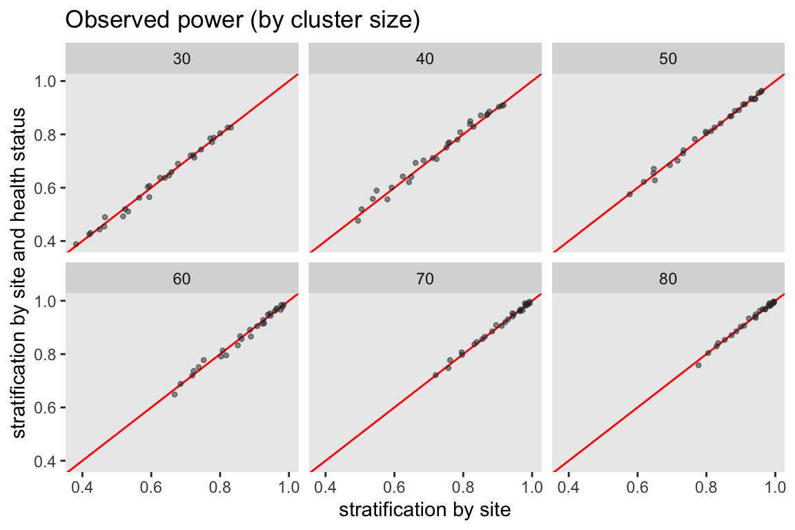
The plots below compare the estimates of the two different stratification strategies. Each point represents a specific scenario under stratification by site alone and stratification by site along and health status. If there are differences in the two strategies, we would expect to see the points diverge from the horizontal line. For all four plots, there appears to be little if any divergence, suggesting that, for these scenarios at least, little difference between stratification scenarios.
Power
In this first scatter plot, the estimated power under each stratification strategy is plotted. Power is estimated by the proportion of p-values in the 2500 iterations that were less than 0.05. Regardless of whether observed power for a particular scenario is high or low, we generally observe the same power under both strategies. The points do not diverge far from the red line, which represents perfect equality.
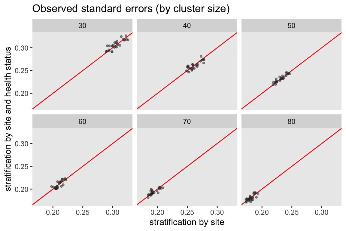
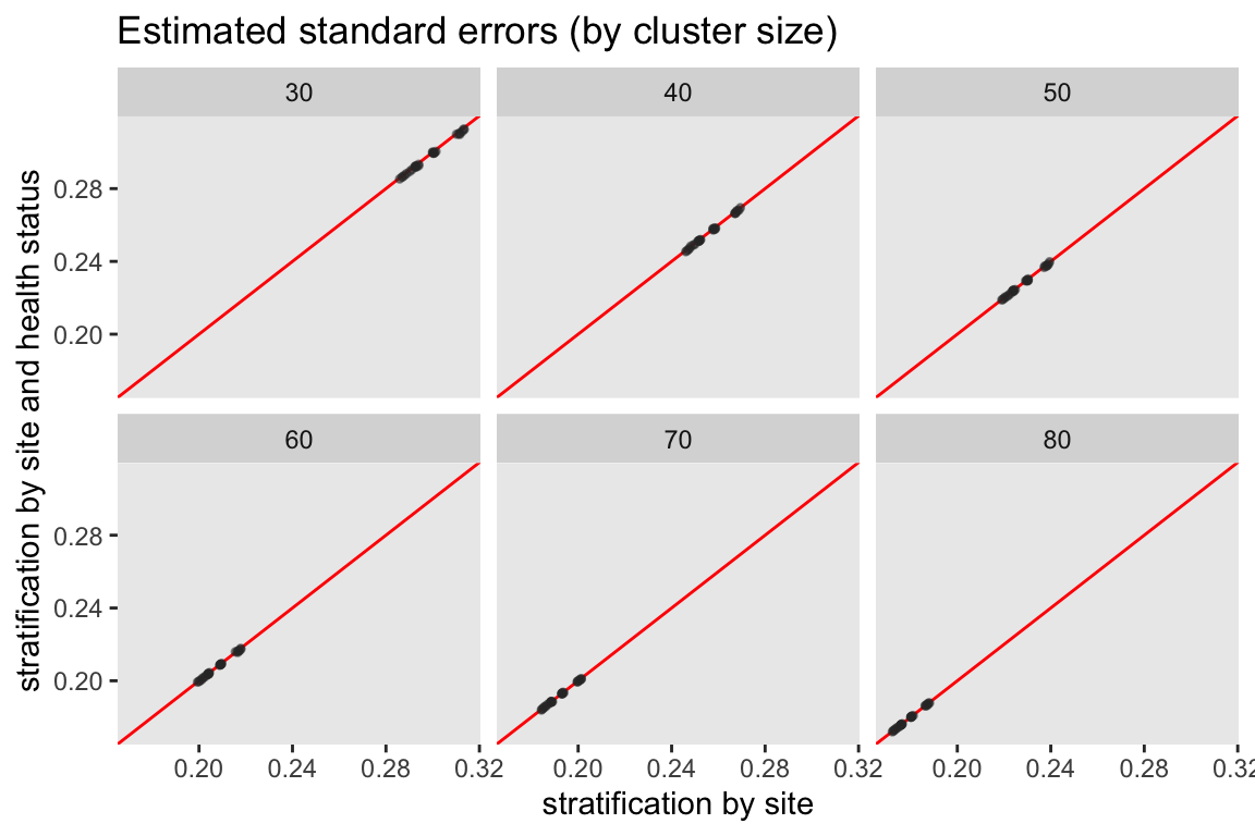
Standard errors
There are two ways to look at the variability of the two strategies. First, we can look at the observed variability of the effect estimates across the 2500 iterations. And second, we can look at the average of the standard error estimates across the iterations. In general, the two randomization schemes appear quite similar with respect to both observed and estimated variation.
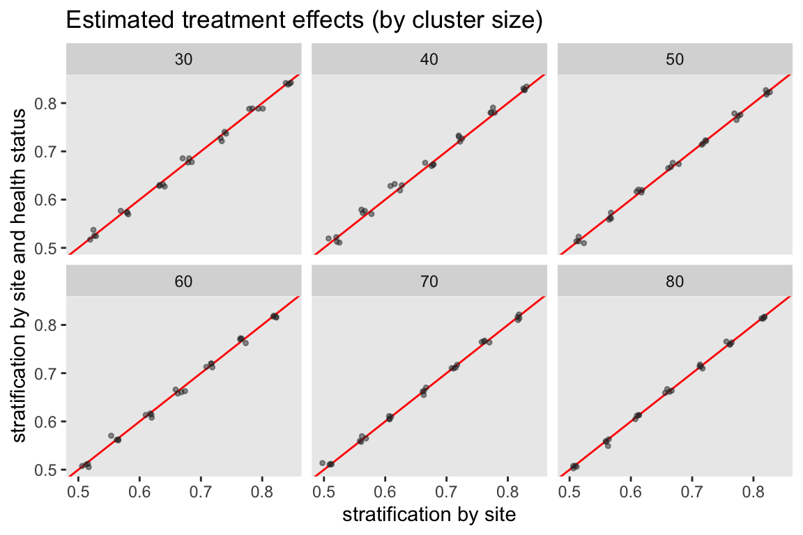
Treatment effects
In this last plot, the average estimated treatment effect is shown for each scenario. The two stratification strategies both appear to provide the same unbiased estimates of the treatment effect.
References:
Kernan, Walter N., Catherine M. Viscoli, Robert W. Makuch, Lawrence M. Brass, and Ralph I. Horwitz. “Stratified randomization for clinical trials.” Journal of clinical epidemiology 52, no. 1 (1999): 19-26.