Generating and modeling over-dispersed binomial data

A count outcome

In this study, one of the primary outcomes is the number of days of opioid use over a six-month follow-up period (to be recorded monthly by patient-report and aggregated for the six-month measure). While one might get away with assuming that the outcome is continuous, it really is not; it is a count outcome, and the possible range is 0 to 180. There are two related questions here - what model will be used to analyze the data once the study is complete? And, how should we generate simulated data to estimate the power of the study?

In this particular study, the randomization is at the physician level so that all patients in a particular physician practice will be in control or treatment. (For the purposes of simplification here, I am going to assume there is no treatment effect, so that all variation in the outcome is due to physicians and patients only.) One possibility is to assume the outcome \(Y_{ij}\) for patient \(i\) in group \(j\) has a binomial distribution with 180 different “experiments” - every day we ask did the patient use opioids? - so that we say \(Y_{ij} \sim Bin(180, \ p_{ij})\).

The probability parameter

The key parameter here is \(p_{ij}\), the probability that patient \(i\) (in group \(j\)) uses opioids on any given day. Given the binomial distribution, the number of days of opioid use we expect to observe for patient \(i\) is \(180p_{ij}\). There are at least three ways to think about how to model this probability (though there are certainly more):

• \(p_{ij} = p\): everyone shares the same probability The collection of all patients will represent a sample from \(Bin(180, p)\).
• \(p_{ij} = p_j\): the probability of the outcome is determined by the cluster or group alone. The data within the cluster will have a binomial distribution, but the collective data set will not have a strict binomial distribution and will be over-dispersed.
• \(p_{ij}\) is unique for each individual. Once again the collective data are over-dispersed, potentially even more so.

Modeling the outcome

The correct model depends, of course, on the situation at hand. What data generation process fits what we expect to be the case? Hopefully, there are existing data to inform the likely model. If not, it may by most prudent to be conservative, which usually means assuming more variation (unique \(p_{ij}\)) rather than less (\(p_{ij} = p\)).

In the first case, the probability (and counts) can be estimated using a generalized linear model (GLM) with a binomial distribution. In the second, one solution (that I will show here) is a generalized linear mixed effects model (GLMM) with a binomial distribution and a group level random effect. In the third case, a GLMM with a negative a negative binomial distribution would be more likely to properly estimate the variation. (I have described other ways to think about these kind of data here and here.)

Case 1: binomial distribution

Even though there is no clustering effect in this first scenario, let’s assume there are clusters. Each individual will have a probability of 0.4 of using opioids on any given day (log odds = -0.405):

def <- defData(varname = "m", formula = 100, dist = "nonrandom", id = "cid")

defa <- defDataAdd(varname = "x", formula = -.405, variance = 180, 
                   dist = "binomial", link = "logit")

Generate the data:

set.seed(5113373)

dc <- genData(200, def)
dd <- genCluster(dc, cLevelVar = "cid", numIndsVar = "m", level1ID = "id")
dd <- addColumns(defa, dd)

Here is a plot of 20 of the 100 groups:

dplot <- dd[cid %in% c(1:20)]
davg <- dplot[, .(avgx = mean(x)), keyby = cid]

ggplot(data=dplot, aes(y = x, x = factor(cid))) +
  geom_jitter(size = .5, color = "grey50", width = 0.2) +
  geom_point(data = davg, aes(y = avgx, x = factor(cid)), 
             shape = 21, fill = "firebrick3", size = 2) +
  theme(panel.grid.major.y = element_blank(),
        panel.grid.minor.y = element_blank(),
        axis.ticks.x = element_blank(),
        axis.text.x = element_blank()
  ) +
  xlab("Group") +
  scale_y_continuous(limits = c(0, 185), breaks = c(0, 60, 120, 180))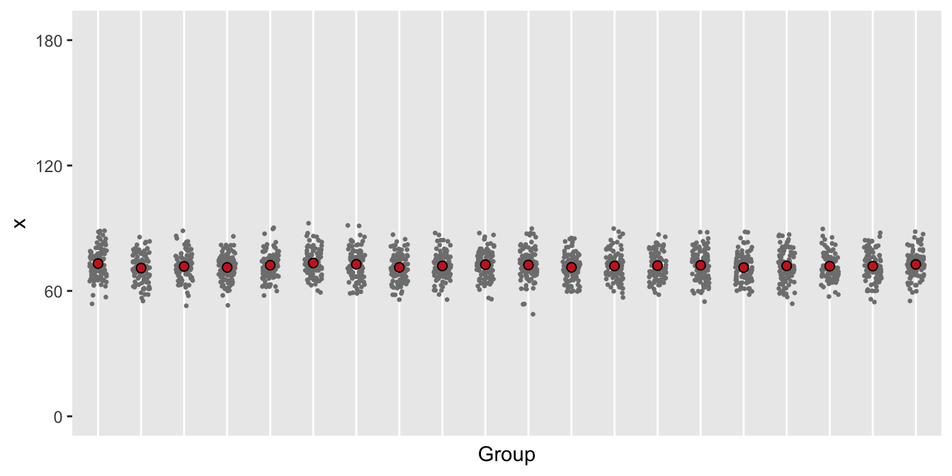

Looking at the plot, we can see that a mixed effects model is probably not relevant.

Case 2: over-dispersion from clustering

def <- defData(varname = "ceffect", formula = 0, variance = 0.08, 
               dist = "normal", id = "cid")
def <- defData(def, varname = "m", formula = "100", dist = "nonrandom")

defa <- defDataAdd(varname = "x", formula = "-0.405 + ceffect", 
                   variance = 100, dist = "binomial", link = "logit")

dc <- genData(200, def)
dd <- genCluster(dc, cLevelVar = "cid", numIndsVar = "m", level1ID = "id")
dd <- addColumns(defa, dd)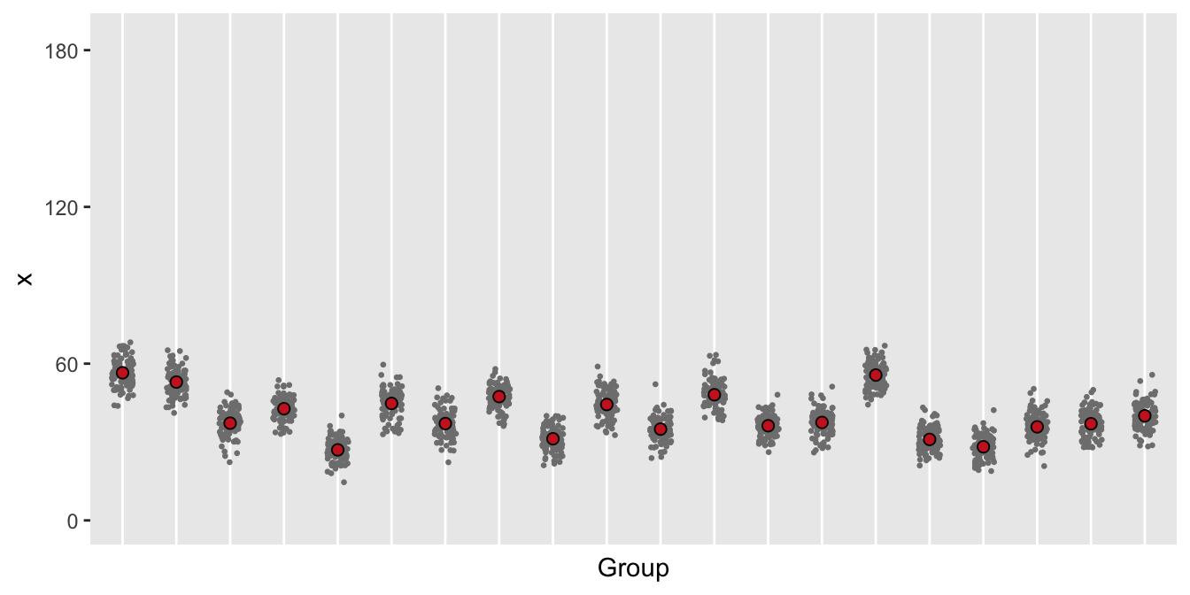

This plot suggests that variation within the groups is pretty consistent, though there is variation across the groups. This suggests that a binomial GLMM with a group level random effect would be appropriate.

Case 3: added over-dispersion due to individual differences

defa <- defDataAdd(varname = "ieffect", formula = 0, 
                   variance = .25, dist = "normal")
defa <- defDataAdd(defa, varname = "x", 
                   formula = "-0.405 + ceffect + ieffect", 
                   variance = 180, dist = "binomial", link = "logit")

dd <- genCluster(dc, cLevelVar = "cid", numIndsVar = "m", level1ID = "id")
dd <- addColumns(defa, dd)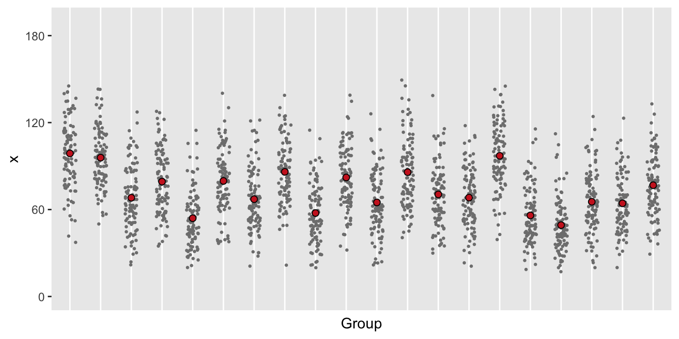

In this last case, it is not obvious what model to use. Since there is variability within and between groups, it is probably safe to use a negative binomial model, which is most conservative.

Estimating the parameters under a negative binomial assumption

We can fit the data we just generated (with a 2-level mixed effects model) using a single-level mixed effects model with the assumption of a negative binomial distribution to estimate the parameters we can use for one last simulated data set. Here is the model fit:

nbfit <- glmer.nb(x ~ 1 + (1|cid), data = dd, 
                    control = glmerControl(optimizer="bobyqa"))
broom::tidy(nbfit)

## # A tibble: 2 x 6
##   term               estimate std.error statistic p.value group
##   <chr>                 <dbl>     <dbl>     <dbl>   <dbl> <chr>
## 1 (Intercept)           4.29     0.0123      347.       0 fixed
## 2 sd_(Intercept).cid    0.172   NA            NA       NA cid

And to generate the negative binomial data using simstudy, we need a dispersion parameter, which can be extracted from the estimated model:

(theta <- 1/getME(nbfit, "glmer.nb.theta"))

## [1] 0.079

revar <-  lme4::getME(nbfit, name = "theta")^2
revar

## cid.(Intercept) 
##            0.03

Generating the data from the estimated model allows us to see how well the negative binomial model fit the dispersed binomial data that we generated. A plot of the two data sets should look pretty similar, at least with respect to the distribution of the cluster means and within-cluster individual counts.

def <- defData(varname = "ceffect", formula = 0, variance = revar, 
               dist = "normal", id = "cid")
def <- defData(def, varname = "m", formula = "100", dist = "nonrandom")

defa <- defDataAdd(varname = "x", formula = "4.28 + ceffect", 
                   variance = theta, dist = "negBinomial", link = "log")

dc <- genData(200, def)
ddnb <- genCluster(dc, cLevelVar = "cid", numIndsVar = "m", 
                   level1ID = "id")
ddnb <- addColumns(defa, ddnb)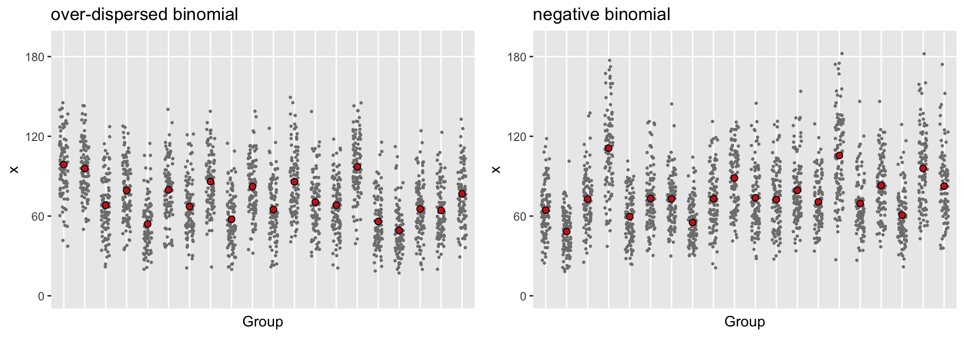

The two data sets do look like they came from the same distribution. The one limitation of the negative binomial distribution is that the sample space is not limited to numbers between 0 and 180; in fact, the sample space is all non-negative integers. For at least two clusters shown, there are some individuals with counts that exceed 180 days, which of course is impossible. Because of this, it might be safer to use the over-dispersed binomial data as the generating process for a power calculation, but it would be totally fine to use the negative binomial model as the analysis model (in both the power calculation and the actual data analysis).

Estimating power

One could verify that power is indeed reduced as we move from Case 1 to Case 3. (I’ll leave that as an exercise for you - I think I’ve provided many examples in the past on how one might go about doing this. If, after struggling for a while, you aren’t successful, feel free to get in touch with me.)