A minor update to simstudy provides an excuse to talk a bit about the negative binomial and Poisson distributions

Added variation

In many situations, when count data are modeled, it turns out that the variance of the data exceeds the mean (a situation called over-dispersion). In this case an alternative model is used that allows for the greater variance, which is based on the negative binomial distribution. It turns out that if the negative binomial distribution has mean \(\mu\), it has a variance of \(\mu + \theta \mu^2\), where \(\theta\) is called a dispersion parameter. If \(\theta = 0\), we have the Poisson distribution, but otherwise the variance of a negative binomial random variable will exceed the variance of a Poisson random variable as long as they share the same mean, because \(\mu > 0\) and \(\theta \ge 0\).

We can see this by generating data from each distribution with mean 15, and a dispersion parameter of 0.2 for the negative binomial. We expect a variance around 15 for the Poisson distribution, and 60 for the negative binomial distribution.

library(simstudy)
library(ggplot2)

# for a less cluttered look

theme_no_minor <- function(color = "grey90") {    
  theme(panel.grid.minor = element_blank(),
        panel.background = element_rect(fill="grey95")
  )
}

options(digits = 2)

# define data

defC <- defCondition(condition = "dist == 0", formula = 15, 
                     dist = "poisson", link = "identity")

defC <- defCondition(defC, condition = "dist == 1", formula = 15, 
                     variance = 0.2, dist = "negBinomial", 
                     link = "identity")

# generate data

set.seed(50)
dt <- genData(500)
dt <- trtAssign(dt, 2, grpName = "dist")
dt <- addCondition(defC, dt, "y")
genFactor(dt, "dist", c("Poisson", "Negative binomial"))

# compare distributions

dt[, .(mean = mean(y), var = var(y)), keyby = fdist]

##                fdist mean var
## 1:           Poisson   15  15
## 2: Negative binomial   15  54

ggplot(data = dt, aes(x = y, group = fdist)) +
  geom_density(aes(fill=fdist), alpha = .4) +
  scale_fill_manual(values = c("#808000", "#000080")) +
  scale_x_continuous(limits = c(0,60), 
                     breaks = seq(0, 60, by = 20)) +
  theme_no_minor() +
  theme(legend.title = element_blank(),
        legend.position = c(0.80, 0.83))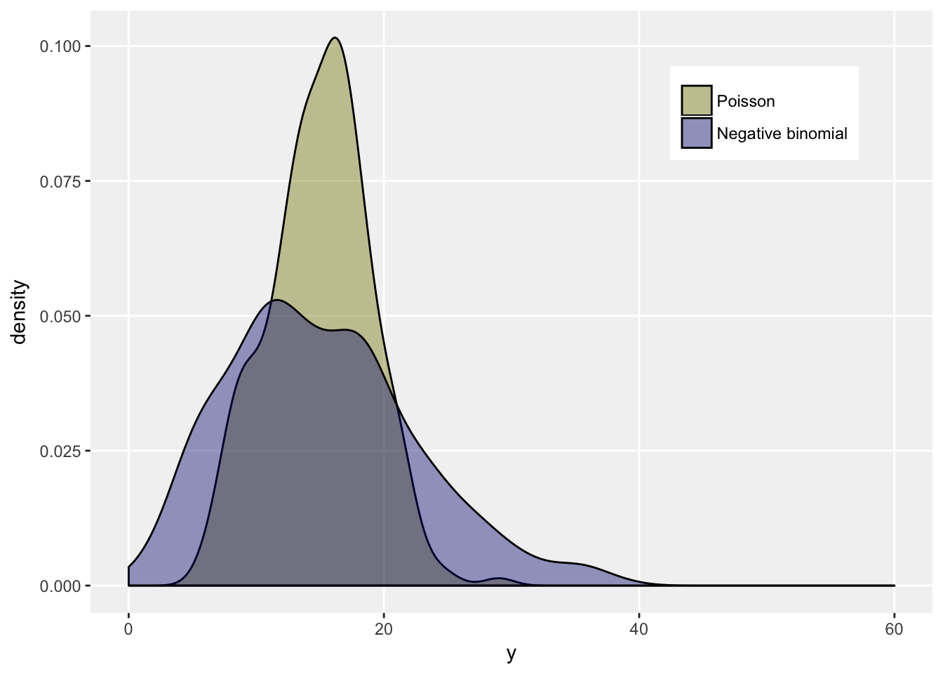

Underestimating standard errors

In the context of a regression, misspecifying a model as Poisson rather than negative binomial, can lead to an underestimation of standard errors, even though the point estimates may be quite reasonable (or may not). The Poisson model will force the variance estimate to be equal to the mean at any particular point on the regression curve. The Poisson model will effectively ignore the true extent of the variation, which can lead to problems of interpretation. We might conclude that there is an association when in fact there is none.

In this simple simulation, we generate two predictors (\(x\) and \(b\)) and an outcome (\(y\)). The outcome is a function of \(x\) only:

library(broom)
library(MASS)

# Generating data from negative binomial dist

def <- defData(varname = "x", formula = 0, variance = 1, 
               dist = "normal")
def <- defData(def, varname = "b", formula = 0, variance = 1, 
               dist = "normal")
def <- defData(def, varname = "y", formula = "0.9 + 0.6*x", 
               variance = 0.3, dist = "negBinomial", link = "log")

set.seed(35)
dt <- genData(500, def)

ggplot(data = dt, aes(x=x, y = y)) +
  geom_jitter(width = .1) +
  ggtitle("Outcome as function of 1st predictor") +
  theme_no_minor()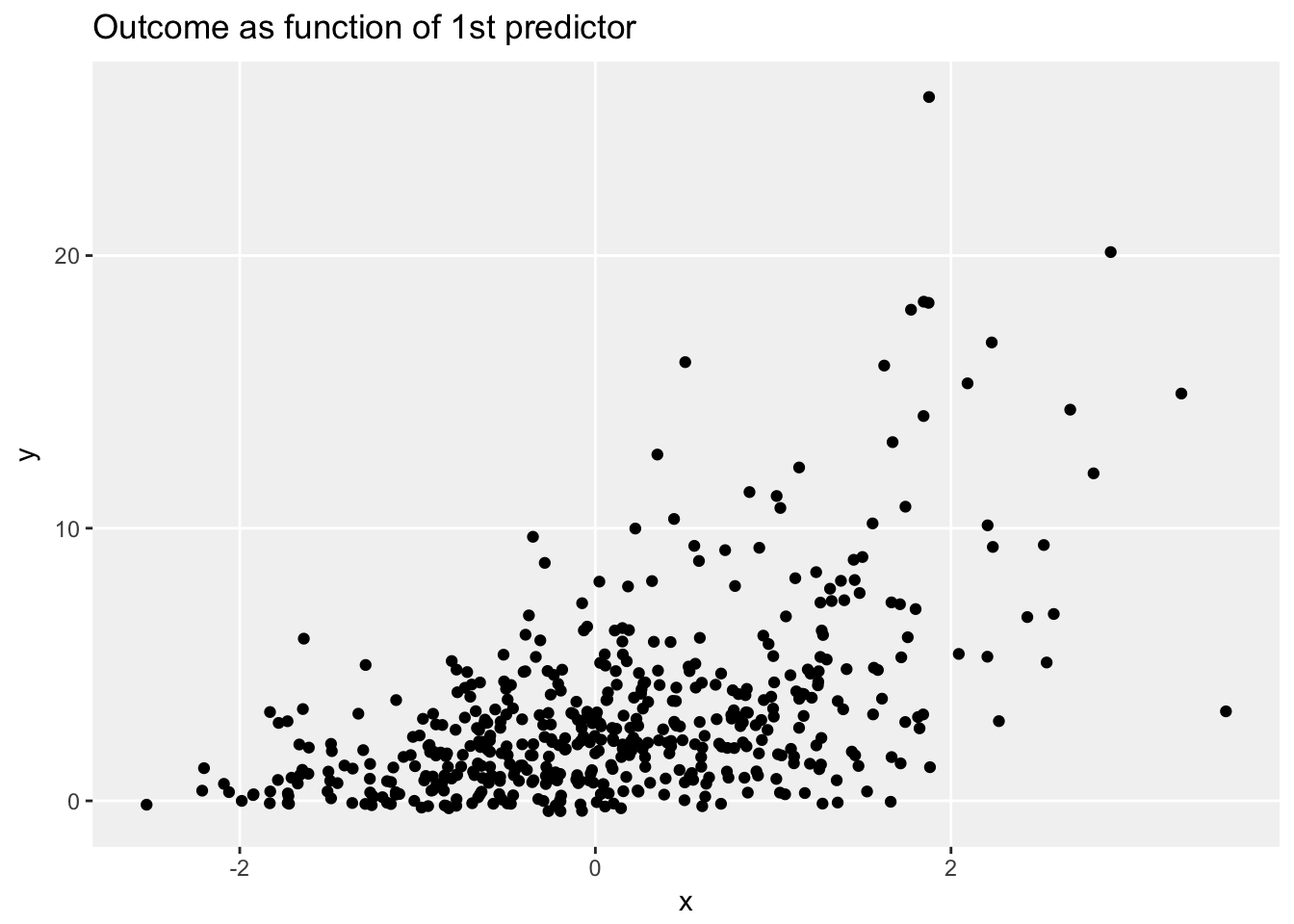

ggplot(data = dt, aes(x=b, y = y)) +
  geom_jitter(width = 0) +
  ggtitle("Outcome as function of 2nd predictor") +
  theme_no_minor()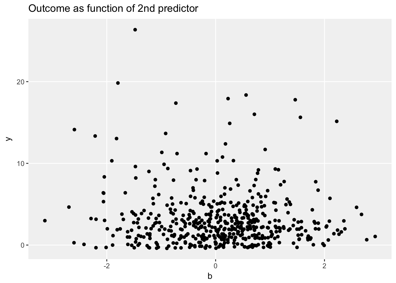

I fit two models using both predictors. The first assumes (incorrectly) a Poisson distribution, and the second assumes (correctly) a negative binomial distribution. We can see that although the point estimates are quite close, the standard error estimates for the predictors in the Poisson model are considerably greater (about 50% higher) than the negative binomial model. And if we were basing any conclusion on the p-value (which is not always the obvious way to do things), we might make the wrong call since the p-value for the slope of \(b\) is estimated to be 0.029. Under the correct model model, the p-value is 0.29.

glmfit <- glm(y ~ x + b, data = dt, family = poisson (link = "log") )
tidy(glmfit)

##          term estimate std.error statistic  p.value
## 1 (Intercept)    0.956     0.030      32.3 1.1e-228
## 2           x    0.516     0.024      21.9 1.9e-106
## 3           b   -0.052     0.024      -2.2  2.9e-02

nbfit <- glm.nb(y ~ x + b, data = dt)
tidy(nbfit)

##          term estimate std.error statistic  p.value
## 1 (Intercept)    0.954     0.039      24.2 1.1e-129
## 2           x    0.519     0.037      14.2  7.9e-46
## 3           b   -0.037     0.036      -1.1  2.9e-01

A plot of the fitted regression curve and confidence bands of \(b\) estimated by each model reinforces the difference. The lighter shaded region is the wider confidence band of the negative binomial model, and the darker shaded region the based on the Poisson model.

newb <- data.table(b=seq(-3,3,length = 100), x = 0)

poispred <- predict(glmfit, newdata = newb, se.fit = TRUE, 
                    type = "response")
nbpred <-predict(nbfit, newdata = newb, se.fit = TRUE, 
                 type = "response")

poisdf <- data.table(b = newb$b, y = poispred$fit, 
                     lwr = poispred$fit - 1.96*poispred$se.fit,
                     upr = poispred$fit + 1.96*poispred$se.fit)

nbdf <- data.table(b = newb$b,  y = nbpred$fit, 
                     lwr = nbpred$fit - 1.96*nbpred$se.fit,
                     upr = nbpred$fit + 1.96*nbpred$se.fit)

ggplot(data = poisdf, aes(x=b, y = y)) +
  geom_line() +
  geom_ribbon(data=nbdf, aes(ymin = lwr, ymax=upr), alpha = .3, 
              fill = "red") +
  geom_ribbon(aes(ymin = lwr, ymax=upr), alpha = .5, 
              fill = "red") +
  theme_no_minor()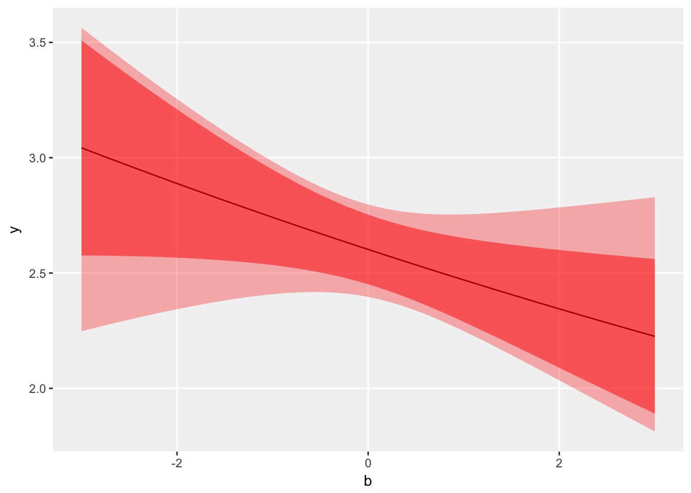

And finally, if we take 500 samples of size 500, and estimate slope for \(b\) each time and calculate the standard deviation of those estimates, it is quite close to the standard error estimate we saw in the model of the original simulated data set using the negative binomial assumption (0.036). And the mean of those estimates is quite close to zero, the true value.

result <- data.table()

for (i in 1:500) {
  
  dt <- genData(500, def)
  glmfit <- glm(y ~ x + b, data = dt, family = poisson)
  nbfit <- glm.nb(y ~ x + b, data = dt)

  result <- rbind(result, data.table(bPois = coef(glmfit)["b"],
                                     bNB = coef(nbfit)["b"])
  )
  
}

result[,.(sd(bPois), sd(bNB))]   # observed standard error

##       V1    V2
## 1: 0.037 0.036

result[,.(mean(bPois), mean(bNB))] # observed mean

##        V1     V2
## 1: 0.0025 0.0033

Negative binomial as mixture of Poissons

An interesting relationship between the two distributions is that a negative binomial distribution can be generated from a mixture of individuals whose outcomes come from a Poisson distribution, but each individual has her own rate or mean. Furthermore, those rates must have a specific distribution - a Gamma. (For much more on this, you can take a look here.) Here is a little simulation:

mu = 15
disp = 0.2

# Gamma distributed means

def <- defData(varname = "gmu", formula = mu, variance = disp, 
               dist = "gamma")

# generate data from each distribution

defC <- defCondition(condition = "nb == 0", formula = "gmu", 
                     dist = "poisson")

defC <- defCondition(defC, condition = "nb == 1", formula = mu,
                     variance = disp, dist = "negBinomial")

dt <- genData(5000, def)
dt <- trtAssign(dt, 2, grpName = "nb")
genFactor(dt, "nb", labels = c("Poisson-Gamma", "Negative binomial"))

dt <- addCondition(defC, dt, "y")

# means and variances should be very close

dt[, .(Mean = mean(y), Var = var(y)), keyby = fnb]

##                  fnb Mean Var
## 1:     Poisson-Gamma   15  62
## 2: Negative binomial   15  57

# plot

ggplot(data = dt, aes(x = y, group = fnb)) +
  geom_density(aes(fill=fnb), alpha = .4) +
  scale_fill_manual(values = c("#808000", "#000080")) +
  scale_x_continuous(limits = c(0,60), 
                     breaks = seq(0, 60, by = 20)) +
  theme_no_minor() +
  theme(legend.title = element_blank(),
        legend.position = c(0.80, 0.83))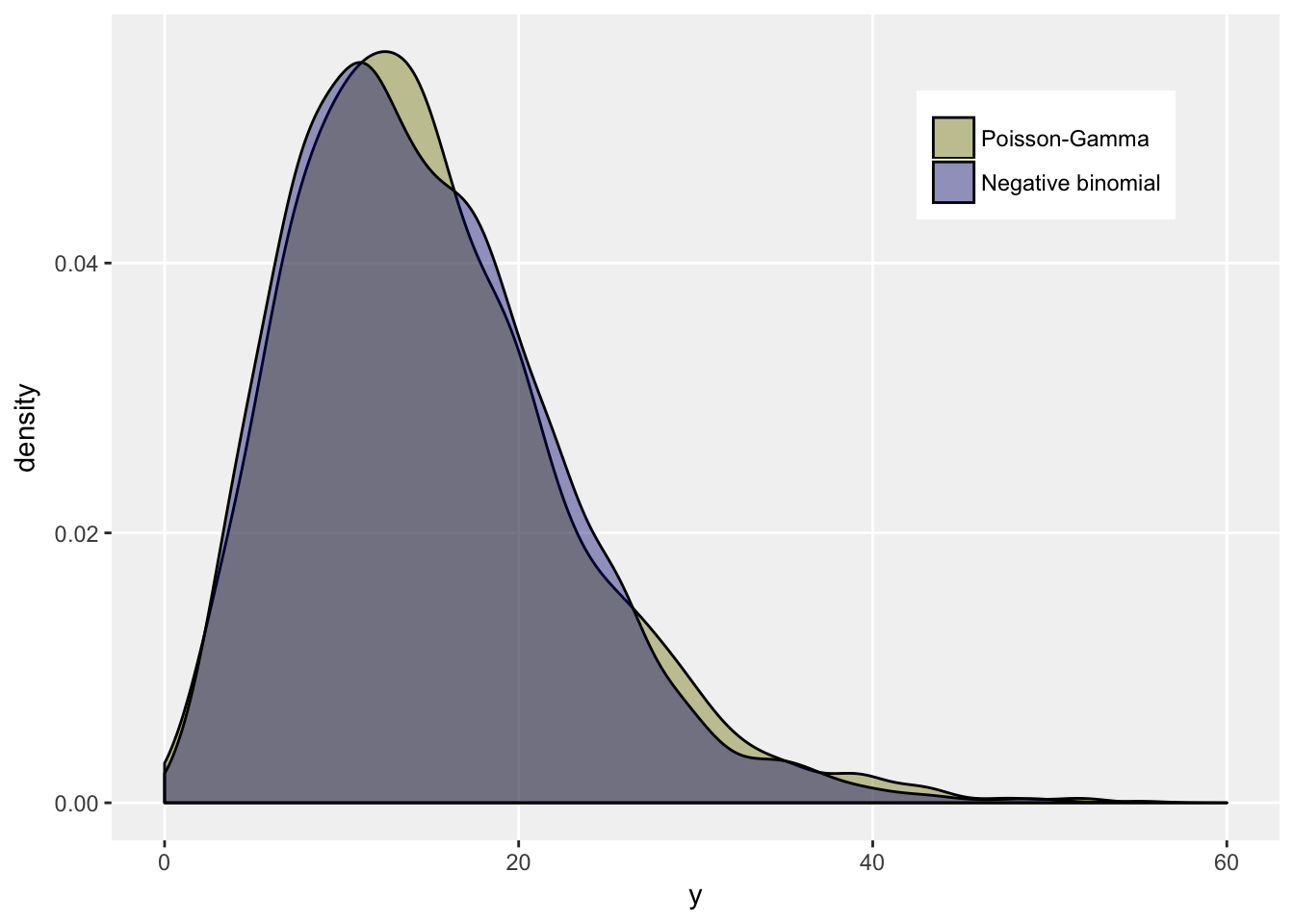

```