Using the simstudy package, it’s possible to generate correlated data from a normal distribution using the function genCorData. I’ve wanted to extend the functionality so that we can generate correlated data from other sorts of distributions; I thought it would be a good idea to begin with binary and Poisson distributed data, since those come up so frequently in my work. simstudy can already accommodate more general correlated data, but only in the context of a random effects data generation process. This might not be what we want, particularly if we are interested in explicitly generating data to explore marginal models (such as a GEE model) rather than a conditional random effects model (a topic I explored in my previous discussion). The extension can quite easily be done using copulas.
Based on this definition, a copula is a “multivariate probability distribution for which the marginal probability distribution of each variable is uniform.” It can be shown that \(U\) is uniformly distributed if \(U=F(X)\), where \(F\) is the CDF of a continuous random variable \(X\). Furthermore, if we can generate a multivariate \(\mathbf{X}\), say \((X_1, X_2, ..., X_k)\) with a known covariance or correlation structure (e.g. exchangeable, auto-regressive, unstructured), it turns that the corresponding multivariate \(\mathbf{U}, (U_1, U_2, ..., U_k)\) will maintain that structure. And in a final step, we can transform \(\mathbf{U}\) to another random variable \(\mathbf{Y}\) that has a target distribution by applying the inverse CDF \(F_i^{-1}(U_i)\) of that target distribution to each \(U_i\). Since we can generate a multivariate normal \(\mathbf{X}\), it is relatively short leap to implement this copula algorithm in order to generate correlated data from other distributions.
Implementing the copula algorithm in R
While this hasn’t been implemented just yet in simstudy, this is along the lines of what I am thinking:
library(simstudy)
library(data.table)

set.seed(555)

# Generate 1000 observations of 4 RVs from a multivariate normal
# dist - each N(0,1) - with a correlation matrix where rho = 0.4

dt <- genCorData(1000, mu = c(0, 0, 0, 0), sigma = 1,
                 rho = 0.4, corstr = "cs" )
dt
## id V1 V2 V3 V4
## 1: 1 -1.1667574 -0.05296536 0.2995360 -0.5232691
## 2: 2 0.4505618 0.57499589 -0.9629426 1.5495697
## 3: 3 -0.1294505 1.68372035 1.1309223 0.4205397
## 4: 4 0.0858846 1.27479473 0.4247491 0.1054230
## 5: 5 0.4654873 3.05566796 0.5846449 1.0906072
## ---
## 996: 996 0.3420099 -0.35783480 -0.8363306 0.2656964
## 997: 997 -1.0928169 0.50081091 -0.8915582 -0.7428976
## 998: 998 0.7490765 -0.09559294 -0.2351121 0.6632157
## 999: 999 0.8143565 -1.00978384 0.2266132 -1.2345192
## 1000: 1000 -1.9795559 -0.16668454 -0.5883966 -1.7424941round(cor(dt[,-1]), 2)## V1 V2 V3 V4
## V1 1.00 0.41 0.36 0.44
## V2 0.41 1.00 0.33 0.42
## V3 0.36 0.33 1.00 0.35
## V4 0.44 0.42 0.35 1.00### create a long version of the data set
dtM <- melt(dt, id.vars = "id", variable.factor = TRUE,
value.name = "X", variable.name = "seq")
setkey(dtM, "id") # sort data by id
dtM[, seqid := .I] # add index for each record
### apply CDF to X to get uniform distribution
dtM[, U := pnorm(X)]
### Generate correlated Poisson data with mean and variance 8
### apply inverse CDF to U
dtM[, Y_pois := qpois(U, 8), keyby = seqid]
dtM## id seq X seqid U Y_pois
## 1: 1 V1 -1.16675744 1 0.12165417 5
## 2: 1 V2 -0.05296536 2 0.47887975 8
## 3: 1 V3 0.29953603 3 0.61773446 9
## 4: 1 V4 -0.52326909 4 0.30039350 6
## 5: 2 V1 0.45056179 5 0.67384729 9
## ---
## 3996: 999 V4 -1.23451924 3996 0.10850474 5
## 3997: 1000 V1 -1.97955591 3997 0.02387673 3
## 3998: 1000 V2 -0.16668454 3998 0.43380913 7
## 3999: 1000 V3 -0.58839655 3999 0.27813308 6
## 4000: 1000 V4 -1.74249414 4000 0.04071101 3### Check mean and variance of Y_pois
dtM[, .(mean = round(mean(Y_pois), 1),
var = round(var(Y_pois), 1)), keyby = seq]## seq mean var
## 1: V1 8.0 8.2
## 2: V2 8.1 8.5
## 3: V3 8.1 7.6
## 4: V4 8.0 7.9### Check correlation matrix of Y_pois's - I know this code is a bit ugly
### but I just wanted to get the correlation matrix quickly.
round(cor(as.matrix(dcast(data = dtM, id~seq,
value.var = "Y_pois")[,-1])), 2)## V1 V2 V3 V4
## V1 1.00 0.40 0.37 0.43
## V2 0.40 1.00 0.33 0.40
## V3 0.37 0.33 1.00 0.35
## V4 0.43 0.40 0.35 1.00The correlation matrices for \(\mathbf{X}\) and \(\mathbf{Y_{Pois}}\) aren’t too far off.
Here are the results for an auto-regressive (AR-1) correlation structure. (I am omitting some of the code for brevity’s sake):
# Generate 1000 observations of 4 RVs from a multivariate normal
# dist - each N(0,1) - with a correlation matrix where rho = 0.4

dt <- genCorData(1000, mu = c(0, 0, 0, 0), sigma = 1,
                 rho = 0.4, corstr = "ar1" )

round(cor(dt[,-1]), 2)
## V1 V2 V3 V4
## V1 1.00 0.43 0.18 0.12
## V2 0.43 1.00 0.39 0.13
## V3 0.18 0.39 1.00 0.38
## V4 0.12 0.13 0.38 1.00### Check mean and variance of Y_pois
dtM[, .(mean = round(mean(Y_pois), 1),
var = round(var(Y_pois), 1)), keyby = seq]## seq mean var
## 1: V1 8.1 8.3
## 2: V2 7.9 7.8
## 3: V3 8.0 8.4
## 4: V4 8.0 7.5### Check correlation matrix of Y_pois's
round(cor(as.matrix(dcast(data = dtM, id~seq,
value.var = "Y_pois")[,-1])), 2)## V1 V2 V3 V4
## V1 1.00 0.41 0.18 0.13
## V2 0.41 1.00 0.39 0.14
## V3 0.18 0.39 1.00 0.36
## V4 0.13 0.14 0.36 1.00Again - comparing the two correlation matrices - the original normal data, and the derivative Poisson data - suggests that this can work pretty well.
Using the last data set, I fit a GEE model to see how well the data generating process is recovered:
library(geepack)

geefit <- geepack::geeglm(Y_pois ~ 1, data = dtM, family = poisson,
                          id = id, corstr = "ar1")

summary(geefit)
##
## Call:
## geepack::geeglm(formula = Y_pois ~ 1, family = poisson, data = dtM,
## id = id, corstr = "ar1")
##
## Coefficients:
## Estimate Std.err Wald Pr(>|W|)
## (Intercept) 2.080597 0.007447 78060 <2e-16 ***
## ---
## Signif. codes: 0 '***' 0.001 '**' 0.01 '*' 0.05 '.' 0.1 ' ' 1
##
## Estimated Scale Parameters:
## Estimate Std.err
## (Intercept) 0.9984 0.02679
##
## Correlation: Structure = ar1 Link = identity
##
## Estimated Correlation Parameters:
## Estimate Std.err
## alpha 0.3987 0.02008
## Number of clusters: 1000 Maximum cluster size: 4In the GEE output, alpha is an estimate of \(\rho\). The estimated alpha is 0.399, quite close to 0.40, the original value used to generate the normally distributed data.
Binary outcomes
We can also generate binary data:
### Generate binary data with p=0.5 (var = 0.25)

dtM[, Y_bin := qbinom(U, 1, .5), keyby = seqid]
dtM
## id seq X seqid U Y_pois Y_bin
## 1: 1 V1 1.7425 1 0.959288 13 1
## 2: 1 V2 1.4915 2 0.932086 12 1
## 3: 1 V3 0.7379 3 0.769722 10 1
## 4: 1 V4 -1.6581 4 0.048644 4 0
## 5: 2 V1 2.3262 5 0.989997 15 1
## ---
## 3996: 999 V4 -0.3805 3996 0.351772 7 0
## 3997: 1000 V1 -0.8724 3997 0.191505 6 0
## 3998: 1000 V2 -1.0085 3998 0.156600 5 0
## 3999: 1000 V3 -2.0451 3999 0.020420 3 0
## 4000: 1000 V4 -2.7668 4000 0.002831 1 0### Check mean and variance of Y_bin
dtM[, .(mean = round(mean(Y_bin), 2),
var = round(var(Y_bin), 2)), keyby = seq]## seq mean var
## 1: V1 0.52 0.25
## 2: V2 0.50 0.25
## 3: V3 0.48 0.25
## 4: V4 0.49 0.25### Check correlation matrix of Y_bin's
round(cor(as.matrix(dcast(data = dtM, id~seq,
value.var = "Y_bin")[,-1])), 2)## V1 V2 V3 V4
## V1 1.00 0.29 0.10 0.05
## V2 0.29 1.00 0.27 0.03
## V3 0.10 0.27 1.00 0.23
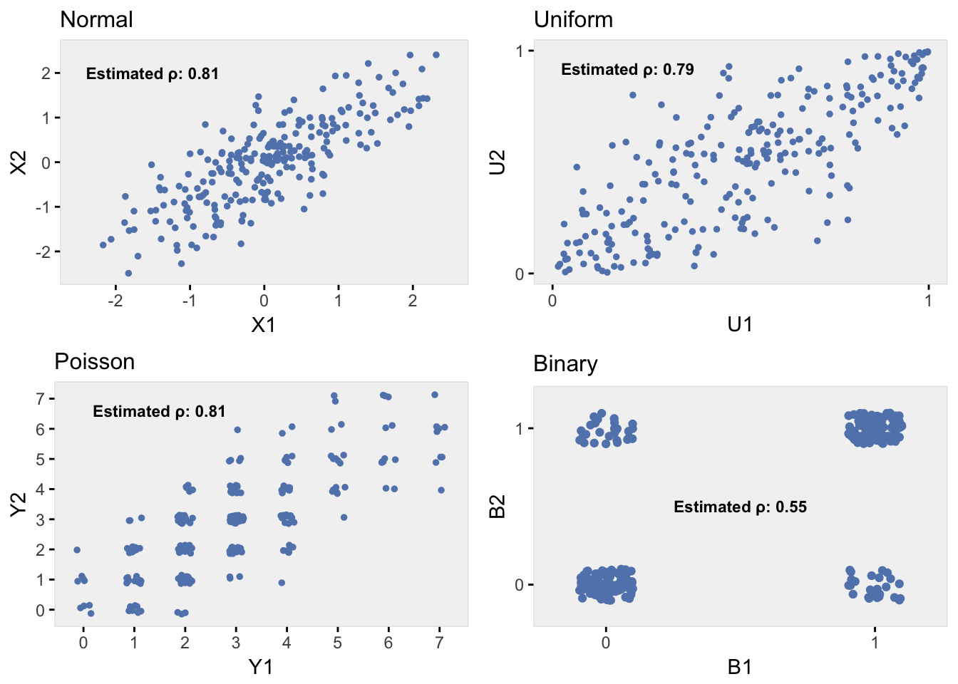
## V4 0.05 0.03 0.23 1.00The binary data are correlated, but the correlation coefficient doesn’t replicate as well as the Poisson distribution. While both the Poisson and binary CDF’s are discontinuous, the extreme jump in the binary CDF leads to this discrepancy. Values that are relatively close to each other on the normal scale, and in particular on the uniform scale, can be ‘sent’ to opposite ends of the binary scale (that is to 0 and to 1) if they straddle the cutoff point \(p\) (the probability of the outcome in the binary distribution); values similar in the original data are very different in the target data. This bias is partially attenuated by values far apart on the uniform scale yet falling on the same side of \(p\) (both driven to 0 or both to 1); in this case values different in the original data are similar (actually identical) in the target data.
The series of plots below show bivariate data for the original multivariate normal data, and the corresponding uniform, Poisson, and binary data. We can see the effect of extreme discontinuity of the binary data. (R code available here.)
Some simulation results
A series of simulations shows how well the estimates of \(\rho\) compare across a set of different assumptions. In each of the plots below, we see how \(\rho\) for the non-normal data changes as a function of \(\rho\) from the original normally distributed data. For each value of \(\rho\), I varied the parameter of the non-normal distribution (in the case of the binary data, I varied the probability of the outcome; in the case of the Poisson data, I varied the parameter \(\lambda\) which defines the mean and variance). I also considered both covariance structures, exchangeable and ar-1. (R code available here.)
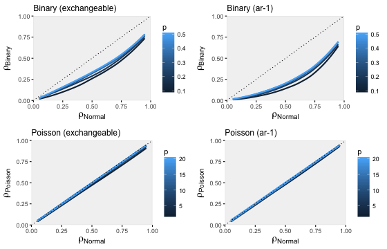
These simulations confirm what we saw earlier. The Poisson data generating process recovers the original \(\rho\) under both covariance structures reasonably well. The binary data generating process is less successful, with the exchangeable structure doing slightly better than then auto-regressive structure.
Hopefully soon, this will be implemented in simstudy so that we can generate data from more general distributions with a single function call.