A key motivating factor for the simstudy package and much of this blog is that simulation can be super helpful in understanding how best to approach an unusual, or least unfamiliar, analytic problem. About six months ago, I described the DREAM Initiative (Diabetes Research, Education, and Action for Minorities), a study that used a slightly innovative randomization scheme to ensure that two comparison groups were evenly balanced across important covariates. At the time, we hadn’t finalized the analytic plan. But, now that we have started actually randomizing and recruiting (yes, in that order, oddly enough), it is important that we do that, with the help of a little simulation.
The study design
The original post has the details about the design and matching algorithm (and code). The randomization is taking place at 20 primary care clinics, and patients within these clinics are matched based on important characteristics before randomization occurs. There is little or no risk that patients in the control arm will be “contaminated” or affected by the intervention that is taking place, which will minimize the effects of clustering. However, we may not want to ignore the clustering altogether.
Possible analytic solutions
Given that the primary outcome is binary, one reasonable procedure to assess whether or not the intervention is effective is McNemar’s test, which is typically used for paired dichotomous data. However, this approach has two limitations. First, McNemar’s test does not take into account the clustered nature of the data. Second, the test is just that, a test; it does not provide an estimate of effect size (and the associated confidence interval).
So, in addition to McNemar’s test, I considered four additional analytic approaches to assess the effect of the intervention: (1) Durkalski’s extension of McNemar’s test to account for clustering, (2) conditional logistic regression, which takes into account stratification and matching, (3) standard logistic regression with specific adjustment for the three matching variables, and (4) mixed effects logistic regression with matching covariate adjustment and a clinic-level random intercept. (In the mixed effects model, I assume the treatment effect does not vary by site, since I have also assumed that the intervention is delivered in a consistent manner across the sites. These may or may not be reasonable assumptions.)
While I was interested to see how the two tests (McNemar and the extension) performed, my primary goal was to see if any of the regression models was superior. In order to do this, I wanted to compare the methods in a scenario without any intervention effect, and in another scenario where there was an effect. I was interested in comparing bias, error rates, and variance estimates.
Data generation
The data generation process parallels the earlier post. The treatment assignment is made in the context of the matching process, which I am not showing this time around. Note that in this initial example, the outcome y depends on the intervention rx (i.e. there is an intervention effect).
library(simstudy)

### defining the data

defc <- defData(varname = "ceffect", formula = 0, variance = 0.4,
                dist = "normal", id = "cid")

defi <- defDataAdd(varname = "male", formula = .4, dist = "binary")
defi <- defDataAdd(defi, varname = "age", formula = 0, variance = 40)
defi <- defDataAdd(defi, varname = "bmi", formula = 0, variance = 5)

defr <- defDataAdd(varname = "y",
  formula = "-1 + 0.08*bmi - 0.3*male - 0.08*age + 0.45*rx + ceffect",
  dist = "binary", link = "logit")

### generating the data

set.seed(547317)

dc <- genData(20, defc)

di <- genCluster(dc, "cid", 60, "id")
di <- addColumns(defi, di)

### matching and randomization within cluster (cid)

library(parallel)
library(Matching)

RNGkind("L'Ecuyer-CMRG")  # to set seed for parallel process

### See addendum for dmatch code

dd <- rbindlist(mclapply(1:nrow(dc),
                         function(x) dmatch(di[cid == x]),
                         mc.set.seed = TRUE
                         )
                )

### generate outcome

dd <- addColumns(defr, dd)
setkey(dd, pair)
dd
## cid ceffect id male age bmi rx pair y
## 1: 1 1.168 11 1 4.35 0.6886 0 1.01 1
## 2: 1 1.168 53 1 3.85 0.2215 1 1.01 1
## 3: 1 1.168 51 0 6.01 -0.9321 0 1.02 0
## 4: 1 1.168 58 0 7.02 0.1407 1 1.02 1
## 5: 1 1.168 57 0 9.25 -1.3253 0 1.03 1
## ---
## 798: 9 -0.413 504 1 -8.72 -0.0767 1 9.17 0
## 799: 9 -0.413 525 0 1.66 3.5507 0 9.18 0
## 800: 9 -0.413 491 0 4.31 2.6968 1 9.18 0
## 801: 9 -0.413 499 0 7.36 0.6064 0 9.19 0
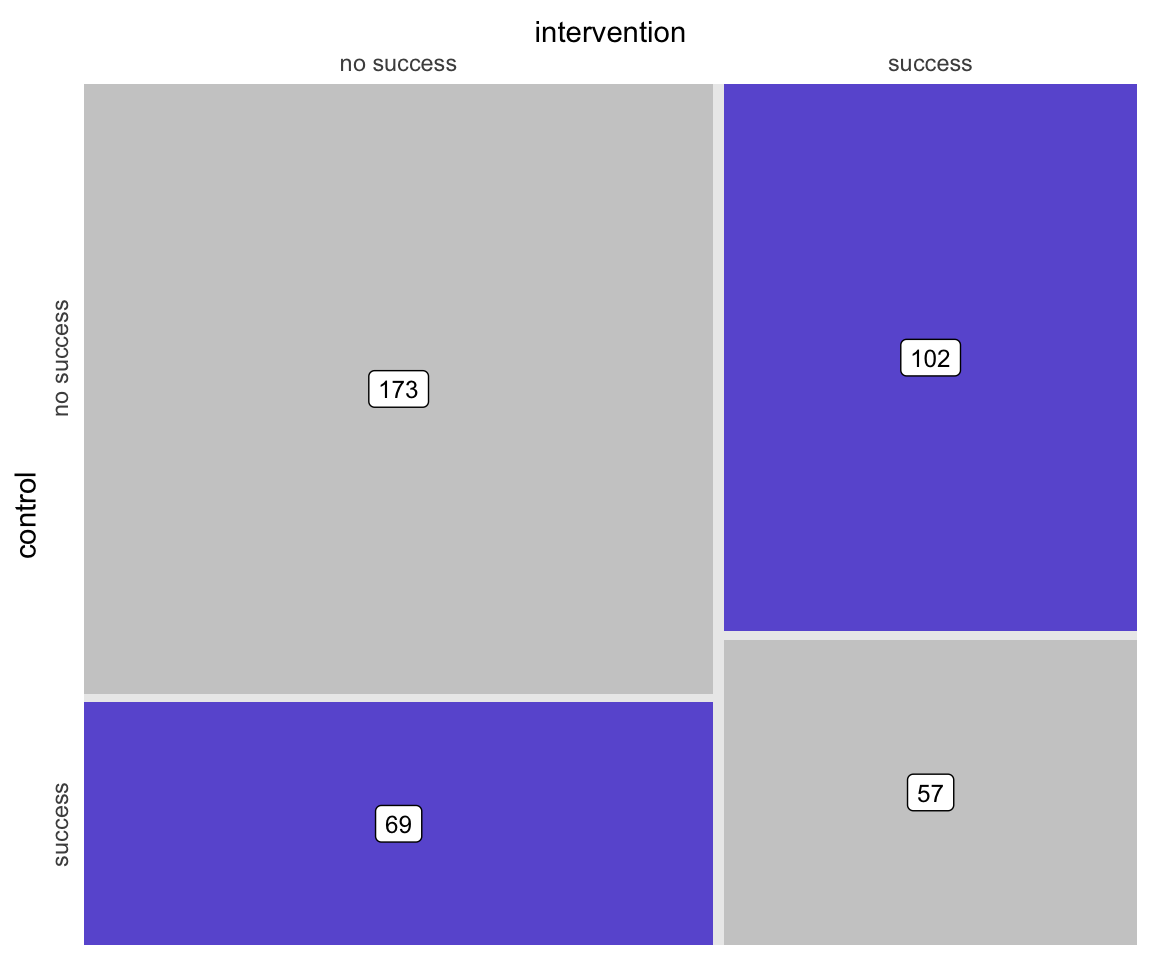
## 802: 9 -0.413 531 0 8.05 0.8068 1 9.19 0Based on the outcomes of each individual, each pair can be assigned to a particular category that describes the outcomes. Either both fail, both succeed, or one fails and the other succeeds. These category counts can be represented in a \(2 \times 2\) contingency table. The counts are the number of pairs in each of the four possible pairwise outcomes. For example, there were 173 pairs where the outcome was determined to be unsuccessful for both intervention and control arms.
dpair <- dcast(dd, pair ~ rx, value.var = "y")
dpair[, control := factor(`0`, levels = c(0,1),
                          labels = c("no success", "success"))]
dpair[, rx := factor(`1`, levels = c(0, 1),
                     labels = c("no success", "success"))]

dpair[, table(control,rx)]
## rx
## control no success success
## no success 173 102
## success 69 57Here is a figure that depicts the \(2 \times 2\) matrix, providing a visualization of how the treatment and control group outcomes compare. (The code is in the addendum in case anyone wants to see the lengths I took to make this simple graphic.)
McNemar’s test
McNemar’s test requires the data to be in table format, and the test really only takes into consideration the cells which represent disagreement between treatment arms. In terms of the matrix above, this would be the lower left and upper right quadrants.
ddc <- dcast(dd, pair ~ rx, value.var = "y")
dmat <- ddc[, .N, keyby = .(`0`,`1`)][, matrix(N, 2, 2, byrow = T)]

mcnemar.test(dmat)
##
## McNemar's Chi-squared test with continuity correction
##
## data: dmat
## McNemar's chi-squared = 6, df = 1, p-value = 0.01Based on the p-value = 0.01, we would reject the null hypothesis that the intervention has no effect.
Durkalski extension of McNemar’s test
Durkalski’s test also requires the data to be in tabular form, though there essentially needs to be a table for each cluster. The clust.bin.pair function needs us to separate the table into vectors a, b, c, and d, where each element in each of the vectors is a count for a specific cluster. Vector a is collection of counts for the upper left hand quadrants, b is for the upper right hand quadrants, etc. We have 20 clusters, so each of the four vectors has length 20. Much of the work done in the code below is just getting the data in the right form for the function.
library(clust.bin.pair)

ddc <- dcast(dd, cid + pair ~ rx, value.var = "y")
ddc[, ypair :=  2*`0` + 1*`1`]
dvec <- ddc[, .N, keyby=.(cid, ypair)]
allpossible <- data.table(expand.grid(1:20, 0:3))
setnames(allpossible, c("cid","ypair"))

setkey(dvec, cid, ypair)
setkey(allpossible, cid, ypair)

dvec <- dvec[allpossible]
dvec[is.na(N), N := 0]

a <- dvec[ypair == 0, N]
b <- dvec[ypair == 1, N]
c <- dvec[ypair == 2, N]
d <- dvec[ypair == 3, N]

clust.bin.pair(a, b, c, d, method = "durkalski")
##
## Durkalski's Chi-square test
##
## data: a, b, c, d
## chi-square = 5, df = 1, p-value = 0.03Again, the p-value, though larger, leads us to reject the null.
Conditional logistic regression
Conditional logistic regression is conditional on the pair. Since the pair is similar with respect to the matching variables, no further adjustment (beyond specifying the strata) is necessary.
library(survival)
summary(clogit(y ~ rx + strata(pair), data = dd))$coef["rx",]
## coef exp(coef) se(coef) z Pr(>|z|)
## 0.3909 1.4783 0.1559 2.5076 0.0122
Logistic regression with matching covariates adjustment
Using logistic regression should in theory provide a reasonable estimate of the treatment effect, though given that there is clustering, I wouldn’t expect the standard error estimates to be correct. Although we are not specifically modeling the matching, by including covariates used in the matching, we are effectively estimating a model that is conditional on the pair.
summary(glm(y~rx + age + male + bmi, data = dd,
            family = "binomial"))$coef["rx",]
## Estimate Std. Error z value Pr(>|z|)
## 0.3679 0.1515 2.4285 0.0152
Generalized mixed effects model with matching covariates adjustment
The mixed effects model merely improves on the logistic regression model by ensuring that any clustering effects are reflected in the estimates.
library(lme4)

summary(glmer(y ~ rx + age + male + bmi + (1|cid), data= dd,
              family = "binomial"))$coef["rx",]
## Estimate Std. Error z value Pr(>|z|)
## 0.4030 0.1586 2.5409 0.0111
Comparing the analytic approaches
To compare the methods, I generated 1000 data sets under each scenario. As I mentioned, I wanted to conduct the comparison under two scenarios. The first when there is no intervention effect, and the second with an effect (I will use the effect size used to generate the first data set.
I’ll start with no intervention effect. In this case, the outcome definition sets the true parameter of rx to 0.
defr <- defDataAdd(varname = "y",
  formula = "-1 + 0.08*bmi - 0.3*male - 0.08*age + 0*rx + ceffect",
  dist = "binary", link = "logit")
Using the updated definition, I generate 1000 datasets, and for each one, I apply the five analytic approaches. The results from each iteration are stored in a large list. (The code for the iterative process is shown in the addendum below.) As an example, here are the contents from the 711th iteration:
res[[711]]## $clr
## coef exp(coef) se(coef) z Pr(>|z|)
## rx -0.0263 0.974 0.162 -0.162 0.871
##
## $glm
## Estimate Std. Error z value Pr(>|z|)
## (Intercept) -0.6583 0.1247 -5.279 1.30e-07
## rx -0.0309 0.1565 -0.198 8.43e-01
## age -0.0670 0.0149 -4.495 6.96e-06
## male -0.5131 0.1647 -3.115 1.84e-03
## bmi 0.1308 0.0411 3.184 1.45e-03
##
## $glmer
## Estimate Std. Error z value Pr(>|z|)
## (Intercept) -0.7373 0.1888 -3.91 9.42e-05
## rx -0.0340 0.1617 -0.21 8.33e-01
## age -0.0721 0.0156 -4.61 4.05e-06
## male -0.4896 0.1710 -2.86 4.20e-03
## bmi 0.1366 0.0432 3.16 1.58e-03
##
## $mcnemar
##
## McNemar's Chi-squared test with continuity correction
##
## data: dmat
## McNemar's chi-squared = 0.007, df = 1, p-value = 0.9
##
##
## $durk
##
## Durkalski's Chi-square test
##
## data: a, b, c, d
## chi-square = 0.1, df = 1, p-value = 0.7Summary statistics
To compare the five methods, I am first looking at the proportion of iterations where the p-value is less then 0.05, in which case we would reject the the null hypothesis. (In the case where the null is true, the proportion is the Type 1 error rate; when there is truly an effect, then the proportion is the power.) I am less interested in the hypothesis test than the bias and standard errors, but the first two methods only provide a p-value, so that is all we can assess them on.
Next, I calculate the bias, which is the average effect estimate minus the true effect. And finally, I evaluate the standard errors by looking at the estimated standard error as well as the observed standard error (which is the standard deviation of the point estimates).
pval <- data.frame(
  mcnm = mean(sapply(res, function(x) x$mcnemar$p.value <= 0.05)),
  durk = mean(sapply(res, function(x) x$durk$p.value <= 0.05)),
  clr =mean(sapply(res, function(x) x$clr["rx","Pr(>|z|)"] <= 0.05)),
  glm = mean(sapply(res, function(x) x$glm["rx","Pr(>|z|)"] <= 0.05)),
  glmer = mean(sapply(res, function(x) x$glmer["rx","Pr(>|z|)"] <= 0.05))
)

bias <- data.frame(
  clr = mean(sapply(res, function(x) x$clr["rx", "coef"])),
  glm = mean(sapply(res, function(x) x$glm["rx", "Estimate"])),
  glmer = mean(sapply(res, function(x) x$glmer["rx", "Estimate"]))
)

se <- data.frame(
  clr = mean(sapply(res, function(x) x$clr["rx", "se(coef)"])),
  glm = mean(sapply(res, function(x) x$glm["rx", "Std. Error"])),
  glmer = mean(sapply(res, function(x) x$glmer["rx", "Std. Error"]))
)

obs.se <- data.frame(
  clr = sd(sapply(res, function(x) x$clr["rx", "coef"])),
  glm = sd(sapply(res, function(x) x$glm["rx", "Estimate"])),
  glmer = sd(sapply(res, function(x) x$glmer["rx", "Estimate"]))
)

sumstat <- round(plyr::rbind.fill(pval, bias, se, obs.se), 3)
rownames(sumstat) <- c("prop.rejected", "bias", "se.est", "se.obs")
sumstat
## mcnm durk clr glm glmer
## prop.rejected 0.035 0.048 0.043 0.038 0.044
## bias NA NA 0.006 0.005 0.005
## se.est NA NA 0.167 0.161 0.167
## se.obs NA NA 0.164 0.153 0.164In this first case, where the true underlying effect size is 0, the Type 1 error rate should be 0.05. The Durkalski test, the conditional logistical regression, and the mixed effects model are below that level but closer than the other two methods. All three models provide unbiased point estimates, but the standard logistic regression (glm) underestimates the standard errors. The results from the conditional logistic regression and the mixed effects model are quite close across the board.
Here are the summary statistics for a data set with an intervention effect of 0.45. The results are consistent with the “no effect” simulations, except that the standard linear regression model exhibits some bias. In reality, this is not necessarily bias, but a different estimand. The model that ignores clustering is a marginal model (with respect to the site), whereas the conditional logistic regression and mixed effects models are conditional on the site. (I’ve described this phenomenon here and here.) We are interested in the conditional effect here, so that argues for the conditional models.
The conditional logistic regression and the mixed effects model yielded similar estimates, though the mixed effects model had slightly higher power, which is the reason I opted to use this approach at the end of the day.
##                mcnm  durk   clr    glm  glmer
## prop.rejected 0.766 0.731 0.784  0.766  0.796
## bias             NA    NA 0.000 -0.033 -0.001
## se.est           NA    NA 0.164  0.156  0.162
## se.obs           NA    NA 0.165  0.152  0.162
In this last case, the true underlying data generating process still includes an intervention effect but no clustering. In this scenario, all of the analytic yield similar estimates. However, since there is no guarantee that clustering is not a factor, the mixed effects model will still be the preferred approach.
##                mcnm  durk    clr    glm  glmer
## prop.rejected 0.802 0.774  0.825  0.828  0.830
## bias             NA    NA -0.003 -0.002 -0.001
## se.est           NA    NA  0.159  0.158  0.158
## se.obs           NA    NA  0.151  0.150  0.150
The DREAM Initiative is supported by the National Institutes of Health National Institute of Diabetes and Digestive and Kidney Diseases R01DK11048. The views expressed are those of the author and do not necessarily represent the official position of the funding organizations.
Addendum: multiple datasets and model estimates
gen <- function(nclust, m) {

  dc <- genData(nclust, defc)
  di <- genCluster(dc, "cid", m, "id")
  di <- addColumns(defi, di)

  dr <- rbindlist(mclapply(1:nrow(dc), function(x) dmatch(di[cid == x])))
  dr <- addColumns(defr, dr)

  dr[]

}

iterate <- function(ncluster, m) {

  dd <- gen(ncluster, m)

  clrfit <- summary(clogit(y ~ rx + strata(pair), data = dd))$coef
  glmfit <- summary(glm(y~rx + age + male + bmi, data = dd,
                        family = binomial))$coef
  mefit <- summary(glmer(y~rx + age + male + bmi + (1|cid), data= dd,
                         family = binomial))$coef

  ## McNemar

  ddc <- dcast(dd, pair ~ rx, value.var = "y")
  dmat <- ddc[, .N, keyby = .(`0`,`1`)][, matrix(N, 2, 2, byrow = T)]

  mc <- mcnemar.test(dmat)

  # Clustered McNemar

  ddc <- dcast(dd, cid + pair ~ rx, value.var = "y")
  ddc[, ypair :=  2*`0` + 1*`1`]
  dvec <- ddc[, .N, keyby=.(cid, ypair)]
  allpossible <- data.table(expand.grid(1:20, 0:3))
  setnames(allpossible, c("cid","ypair"))

  setkey(dvec, cid, ypair)
  setkey(allpossible, cid, ypair)

  dvec <- dvec[allpossible]
  dvec[is.na(N), N := 0]

  a <- dvec[ypair == 0, N]
  b <- dvec[ypair == 1, N]
  c <- dvec[ypair == 2, N]
  d <- dvec[ypair == 3, N]

  durk <- clust.bin.pair(a, b, c, d, method = "durkalski")

  list(clr = clrfit, glm = glmfit, glmer = mefit,
       mcnemar = mc, durk = durk)

}

res <- mclapply(1:1000, function(x) iterate(20, 60))
Code to generate figure
library(ggmosaic)

dpair <- dcast(dd, pair ~ rx, value.var = "y")
dpair[, control := factor(`0`, levels = c(1,0),
                          labels = c("success", "no success"))]
dpair[, rx := factor(`1`, levels = c(0, 1),
                     labels = c("no success", "success"))]

p <- ggplot(data = dpair) +
  geom_mosaic(aes(x = product(control, rx)))

pdata <- data.table(ggplot_build(p)$data[[1]])
pdata[, mcnemar := factor(c("diff","same","same", "diff"))]

textloc <- pdata[c(1,4), .(x=(xmin + xmax)/2, y=(ymin + ymax)/2)]

ggplot(data = pdata) +
  geom_rect(aes(xmin=xmin, xmax=xmax, ymin=ymin, ymax=ymax,
                        fill = mcnemar)) +
  geom_label(data = pdata,
          aes(x = (xmin+xmax)/2, y = (ymin+ymax)/2, label=.wt),
          size = 3.2) +
  scale_x_continuous(position = "top",
                     breaks = textloc$x,
                     labels = c("no success", "success"),
                     name = "intervention",
                     expand = c(0,0)) +
  scale_y_continuous(breaks = textloc$y,
                     labels = c("success", "no success"),
                     name = "control",
                     expand = c(0,0)) +
  scale_fill_manual(values = c("#6b5dd5", "grey80")) +
  theme(panel.grid = element_blank(),
        legend.position = "none",
        axis.ticks = element_blank(),
        axis.text.x = element_text(angle = 0, hjust = 0.5),
        axis.text.y = element_text(angle = 90, hjust = 0.5)
  )
Original matching algorithm
dmatch <- function(dsamp) {

  dsamp[, rx := 0]
  dused <- NULL
  drand <- NULL
  dcntl <- NULL

  while (nrow(dsamp) > 1) {

    selectRow <- sample(1:nrow(dsamp), 1)

    dsamp[selectRow, rx := 1]

    myTr <- dsamp[, rx]
    myX <- as.matrix(dsamp[, .(male, age, bmi)])

    match.dt <- Match(Tr = myTr, X = myX,
                      caliper = c(0, 0.50, .50), ties = FALSE)

    if (length(match.dt) == 1) {  # no match

      dused <- rbind(dused, dsamp[selectRow])
      dsamp <- dsamp[-selectRow, ]

    } else {                      # match

      trt <- match.dt$index.treated
      ctl <- match.dt$index.control

      drand <- rbind(drand, dsamp[trt])
      dcntl <- rbind(dcntl, dsamp[ctl])

      dsamp <- dsamp[-c(trt, ctl)]

    }
  }

  dcntl[, pair := paste0(cid, ".", formatC(1:.N, width=2, flag="0"))]
  drand[, pair := paste0(cid, ".", formatC(1:.N, width=2, flag="0"))]

  rbind(dcntl, drand)

}