In health services research, experiments are often conducted at the provider or site level rather than the patient level. However, we might still be interested in the outcome at the patient level. For example, we could be interested in understanding the effect of a training program for physicians on their patients. It would be very difficult to randomize patients to be exposed or not to the training if a group of patients all see the same doctor. So the experiment is set up so that only some doctors get the training and others serve as the control; we still compare the outcome at the patient level.
Typically, when conducting an experiment we assume that individual outcomes are not related to each other (other than the common effect of the exposure). With site-level randomization, we can’t make that assumption - groups of patients are all being treated by the same doctor. In general, even before the intervention, there might be variation across physicians. At the same time, patients within a practice will vary. So, we have two sources of variation: between practice and within practice variation that explain overall variation.
I touched on this when I discussed issues related to Gamma distributed clustered data. A key concept is the intra-class coefficient or ICC, which is a measure of how between variation relates to overall variation. The ICC ranges from 0 (where there is no between variation - all site averages are the same) to 1 (where there is no variation within a site - all patients within the site have the same outcomes). Take a look at the earlier post for a bit more detail.
My goal here is to highlight a little function recently added to simstudy (v0.1.9, now available on CRAN). In the course of exploring study designs for cluster randomized trials, it is often useful to understand what happens (to sample size requirements, for example) when the ICC changes. When generating the data, it is difficult to control the ICC directly - we do this by controlling the variation. With normally distributed data, the ICC is an obvious function of the variances used to generate the data, so the connection is pretty clear. But, when the outcomes have binary, Poisson, or Gamma distributions (or anything else really), the connection between variation and the ICC is not always so obvious. Figuring out how to specify the data to generate a particular ICC might require quite a bit of trial and error.
The new function, iccRE (short for ICC random effects), allows users to specify target ICCs for a desired distribution (along with relevant parameters). The function returns the corresponding random effect variances that would be specified at the cluster level to generate the desired ICC(s).
Here’s an example for three possible ICCs in the context of the normal distribution:
library(simstudy)
library(ggplot2)

targetICC <- c(0.05, 0.075, 0.10)

setVars <- iccRE(ICC = targetICC, dist = "normal", varWithin = 4)

round(setVars, 4)
## [1] 0.2105 0.3243 0.4444In the case when the target ICC is 0.075:
\[ ICC = \frac{\sigma_b^2}{\sigma_b ^2 + \sigma_w ^2} = \frac{0.324}{0.324 + 4} \approx 0.075\]
Simulating from the normal distribution
If we specify the variance for the site-level random effect to be 0.2105 in conjunction with the individual-level (within) variance of 4, the observed ICC from the simulated data will be approximately 0.05:
set.seed(73632)

# specify between site variation

d <- defData(varname = "a", formula = 0, variance = 0.2105, id = "grp")
d <- defData(d, varname = "size", formula = 1000, dist = "nonrandom")

a <- defDataAdd(varname = "y1", formula = "30 + a",
                variance = 4, dist = "normal")

dT <- genData(10000, d)

# add patient level data

dCn05 <- genCluster(dtClust = dT, cLevelVar = "grp",
                 numIndsVar = "size", level1ID = "id")

dCn05 <- addColumns(a, dCn05)
dCn05
## grp a size id y1
## 1: 1 -0.3255465 1000 1 32.08492
## 2: 1 -0.3255465 1000 2 27.21180
## 3: 1 -0.3255465 1000 3 28.37411
## 4: 1 -0.3255465 1000 4 27.70485
## 5: 1 -0.3255465 1000 5 32.11814
## ---
## 9999996: 10000 0.3191311 1000 9999996 30.15837
## 9999997: 10000 0.3191311 1000 9999997 32.66302
## 9999998: 10000 0.3191311 1000 9999998 28.34583
## 9999999: 10000 0.3191311 1000 9999999 28.56443
## 10000000: 10000 0.3191311 1000 10000000 30.06957The between variance can be roughly estimated as the variance of the group means, and the within variance can be estimated as the average of the variances calculated for each group (this works well here, because we have so many clusters and patients per cluster):
between <- dCn05[, mean(y1), keyby = grp][, var(V1)]
within <- dCn05[, var(y1), keyby = grp][, mean(V1)]

total <- dCn05[, var(y1)]

round(c(between, within, total), 3)
## [1] 0.212 3.996 4.203The ICC is the ratio of the between variance to the total, which is also the sum of the two component variances:
round(between/(total), 3)## [1] 0.05round(between/(between + within), 3)## [1] 0.05Setting the site-level variance at 0.4444 gives us the ICC of 0.10:
d <- defData(varname = "a", formula = 0, variance = 0.4444, id = "grp")
d <- defData(d, varname = "size", formula = 1000, dist = "nonrandom")

a <- defDataAdd(varname = "y1", formula = "30 + a",
                variance = 4, dist = "normal")

dT <- genData(10000, d)

dCn10 <- genCluster(dtClust = dT, cLevelVar = "grp",
                 numIndsVar = "size", level1ID = "id")

dCn10 <- addColumns(a, dCn10)

between <- dCn10[, mean(y1), keyby = grp][, var(V1)]
within <- dCn10[, var(y1), keyby = grp][, mean(V1)]

round(between / (between + within), 3)
## [1] 0.102Other distributions
The ICC is a bit more difficult to interpret using other distributions where the variance is a function of the mean, such as with the binomial, Poisson, or Gamma distributions. However, we can still use the notion of between and within, but it may need to be transformed to another scale.
In the case of binary outcomes, we have to imagine an underlying or latent continuous process that takes place on the logistic scale. (I talked a bit about this here.)
### binary

(setVar <- iccRE(ICC = 0.05, dist = "binary"))
## [1] 0.173151d <- defData(varname = "a", formula = 0, variance = 0.1732, id = "grp")
d <- defData(d, varname = "size", formula = 1000, dist = "nonrandom")
a <- defDataAdd(varname = "y1", formula = "-1 + a", dist = "binary",
link = "logit")
dT <- genData(10000, d)
dCb05 <- genCluster(dtClust = dT, cLevelVar = "grp", numIndsVar = "size",
level1ID = "id")
dCb05 <- addColumns(a, dCb05)
dCb05## grp a size id y1
## 1: 1 -0.20740274 1000 1 0
## 2: 1 -0.20740274 1000 2 0
## 3: 1 -0.20740274 1000 3 0
## 4: 1 -0.20740274 1000 4 1
## 5: 1 -0.20740274 1000 5 0
## ---
## 9999996: 10000 -0.05448775 1000 9999996 0
## 9999997: 10000 -0.05448775 1000 9999997 1
## 9999998: 10000 -0.05448775 1000 9999998 0
## 9999999: 10000 -0.05448775 1000 9999999 0
## 10000000: 10000 -0.05448775 1000 10000000 0The ICC for the binary distribution is on the logistic scale, and the within variance is constant. The between variance is estimated on the log-odds scale:
within <- (pi ^ 2) / 3
means <- dCb05[,mean(y1), keyby = grp]
between <- means[, log(V1/(1-V1)), keyby = grp][abs(V1) != Inf, var(V1)]

round(between / (between + within), 3)
## [1] 0.051The ICC for the Poisson distribution is interpreted on the scale of the count measurements, even though the random effect variance is on the log scale. If you want to see the details behind the random effect variance derivation, see this paper by Austin et al., which was based on original work by Stryhn et al. that can be found here.
(setVar <- iccRE(ICC = 0.05, dist = "poisson", lambda = 30))## [1] 0.0017513d <- defData(varname = "a", formula = 0, variance = 0.0018, id = "grp")
d <- defData(d, varname = "size", formula = 1000, dist = "nonrandom")
a <- defDataAdd(varname = "y1", formula = "log(30) + a",
dist = "poisson", link = "log")
dT <- genData(10000, d)
dCp05 <- genCluster(dtClust = dT, cLevelVar = "grp",
numIndsVar = "size", level1ID = "id")
dCp05 <- addColumns(a, dCp05)
dCp05## grp a size id y1
## 1: 1 0.035654485 1000 1 26
## 2: 1 0.035654485 1000 2 36
## 3: 1 0.035654485 1000 3 31
## 4: 1 0.035654485 1000 4 34
## 5: 1 0.035654485 1000 5 21
## ---
## 9999996: 10000 0.002725561 1000 9999996 26
## 9999997: 10000 0.002725561 1000 9999997 25
## 9999998: 10000 0.002725561 1000 9999998 27
## 9999999: 10000 0.002725561 1000 9999999 28
## 10000000: 10000 0.002725561 1000 10000000 37The variance components and ICC for the Poisson can be estimated using the same approach as the normal distribution:
between <- dCp05[, mean(y1), keyby = grp][, var(V1)]
within <- dCp05[, var(y1), keyby = grp][, mean(V1)]

round(between / (between + within), 3)
## [1] 0.051Finally, here are the results for the Gamma distribution, which I talked about in great length in an earlier post:
(setVar <- iccRE(ICC = 0.05, dist = "gamma", disp = 0.25 ))## [1] 0.01493805d <- defData(varname = "a", formula = 0, variance = 0.0149, id = "grp")
d <- defData(d, varname = "size", formula = 1000, dist = "nonrandom")
a <- defDataAdd(varname = "y1", formula = "log(30) + a", variance = 0.25,
dist = "gamma", link = "log")
dT <- genData(10000, d)
dCg05 <- genCluster(dtClust = dT, cLevelVar = "grp", numIndsVar = "size",
level1ID = "id")
dCg05 <- addColumns(a, dCg05)
dCg05## grp a size id y1
## 1: 1 0.09466305 1000 1 14.31268
## 2: 1 0.09466305 1000 2 39.08884
## 3: 1 0.09466305 1000 3 28.08050
## 4: 1 0.09466305 1000 4 53.27853
## 5: 1 0.09466305 1000 5 37.93855
## ---
## 9999996: 10000 0.25566417 1000 9999996 14.16145
## 9999997: 10000 0.25566417 1000 9999997 42.54838
## 9999998: 10000 0.25566417 1000 9999998 76.33642
## 9999999: 10000 0.25566417 1000 9999999 34.16727
## 10000000: 10000 0.25566417 1000 10000000 21.06282The ICC for the Gamma distribution is on the log scale:
between <- dCg05[, mean(log(y1)), keyby = grp][, var(V1)]
within <- dCg05[, var(log(y1)), keyby = grp][, mean(V1)]

round(between / (between + within), 3)
## [1] 0.05It is possible to think about the ICC in the context of covariates, but interpretation is less straightforward. The ICC itself will likely vary across different levels of the covariates. For this reason, I like to think of the ICC in the marginal context.
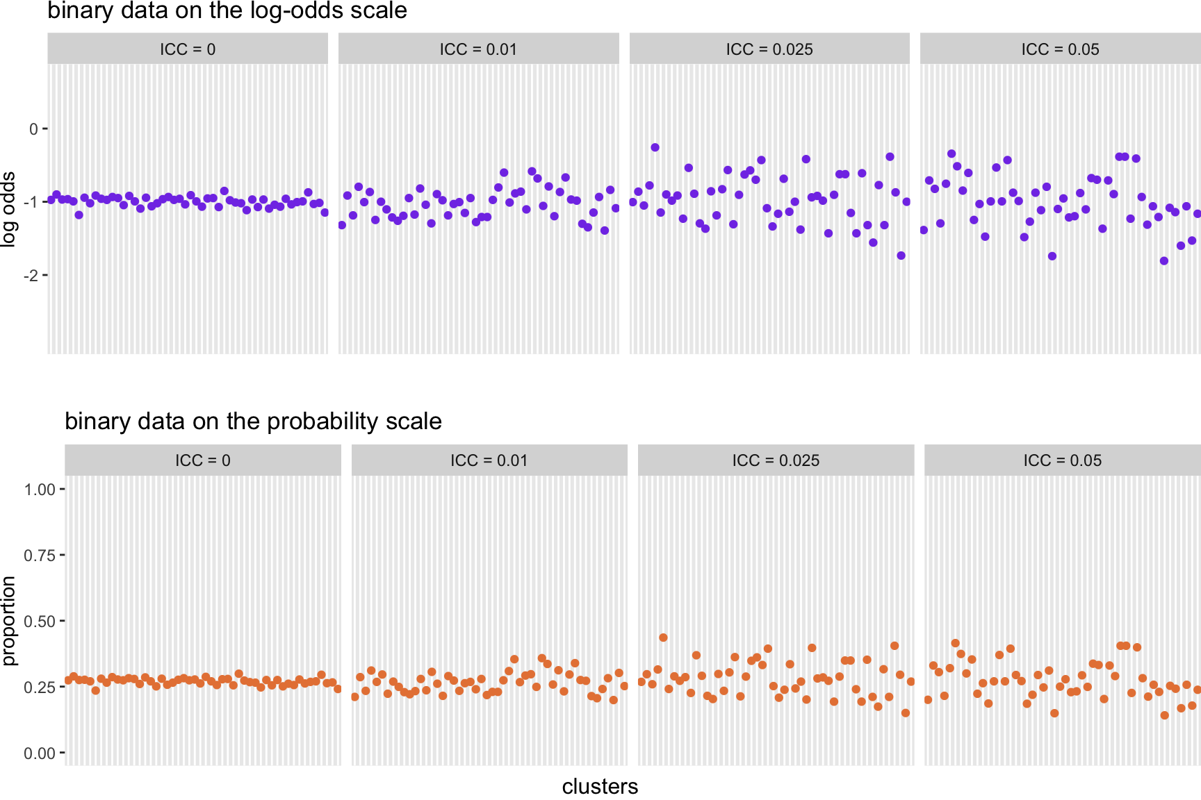
I leave you with some visuals of clustered binary data with ICC’s ranging from 0 to 0.075, both on the log-odds and probability scales: