I was thinking a lot about proportional-odds cumulative logit models last fall while designing a study to evaluate an intervention’s effect on meat consumption. After a fairly extensive pilot study, we had determined that participants can have quite a difficult time recalling precise quantities of meat consumption, so we were forced to move to a categorical response. (This was somewhat unfortunate, because we would not have continuous or even count outcomes, and as a result, might not be able to pick up small changes in behavior.) We opted for a question that was based on 30-day meat consumption: none, 1-3 times per month, 1 time per week, etc. - six groups in total. The question was how best to evaluate effectiveness of the intervention?
Since the outcome was categorical and ordinal - that is category 1 implied less meat consumption that category 2, category 2 implied less consumption that category 3, and so on - a model that estimates the cumulative probability of ordinal outcomes seemed like a possible way to proceed. Cumulative logit models estimate a number of parameters that represent the cumulative log-odds of an outcome; the parameters are the log-odds of categories 2 through 6 versus category 1, categories 3 through 6 versus 1 & 2, etc. Maybe not the most intuitive way to interpret the data, but seems to plausibly fit the data generating process.
I was concerned about the proportionality assumption of the cumulative logit model, particularly when we started to consider adjusting for baseline characteristics (more on that in the next post). I looked more closely at the data generating assumptions of the cumulative logit model, which are quite frequently framed in the context of a continuous latent measure that follows a logistic distribution. I thought I’d describe that data generating process here to give an alternative view of discrete data models.
I know I have been describing a context that includes an outcome with multiple categories, but in this post I will focus on regular logistic regression with a binary outcome. This will hopefully allow me to establish the idea of a latent threshold. I think it will be useful to explain this simpler case first before moving on to the more involved case of an ordinal response variable, which I plan to tackle in the near future.
A latent continuous process underlies the observed binary process
For an event with a binary outcome (true or false, A or B, 0 or 1), the observed outcome may, at least in some cases, be conceived as the manifestation of an unseen, latent continuous outcome. In this conception, the observed (binary) outcome merely reflects whether or not the unseen continuous outcome has exceeded a specified threshold. Think of this threshold as a tipping point, above which the observable characteristic takes on one value (say false), below which it takes on a second value (say true).
The logistic distribution
Logistic regression models are used to estimate relationships of individual characteristics with categorical outcomes. The name of this regression model arises from the logistic distribution, which is a symmetrical continuous distribution. In a latent (or hidden) variable framework, the underlying, unobserved continuous measure is drawn from this logistic distribution. More specifically, the standard logistic distribution is typically assumed, with a location parameter of 0, and a scale parameter of 1. (The mean of this distribution is 0 and variance is approximately 3.29.)
Here is a plot of a logistic pdf, shown in relation to a standard normal pdf (with mean 0 and variance 1):
library(ggplot2)
library(data.table)

my_theme <- function() {
  theme(panel.background = element_rect(fill = "grey90"),
        panel.grid = element_blank(),
        axis.ticks = element_line(colour = "black"),
        panel.spacing = unit(0.25, "lines"),
        plot.title = element_text(size = 12, vjust = 0.5, hjust = 0),
        panel.border = element_rect(fill = NA, colour = "gray90"))
}

x <- seq(-6, 6, length = 1000)
yNorm <- dnorm(x, 0, 1)
yLogis <- dlogis(x, location = 0, scale = 1)

dt <- data.table(x, yNorm, yLogis)
dtm <- melt(dt, id.vars = "x", value.name = "Density")

ggplot(data = dtm) +
  geom_line(aes(x = x, y = Density, color = variable)) +
  geom_hline(yintercept = 0, color = "grey50") +
  my_theme() +
  scale_color_manual(values = c("red", "black"),
                     labels=c("Normal", "Logistic")) +
  theme(legend.position = c(0.8, 0.6),
        legend.title = element_blank())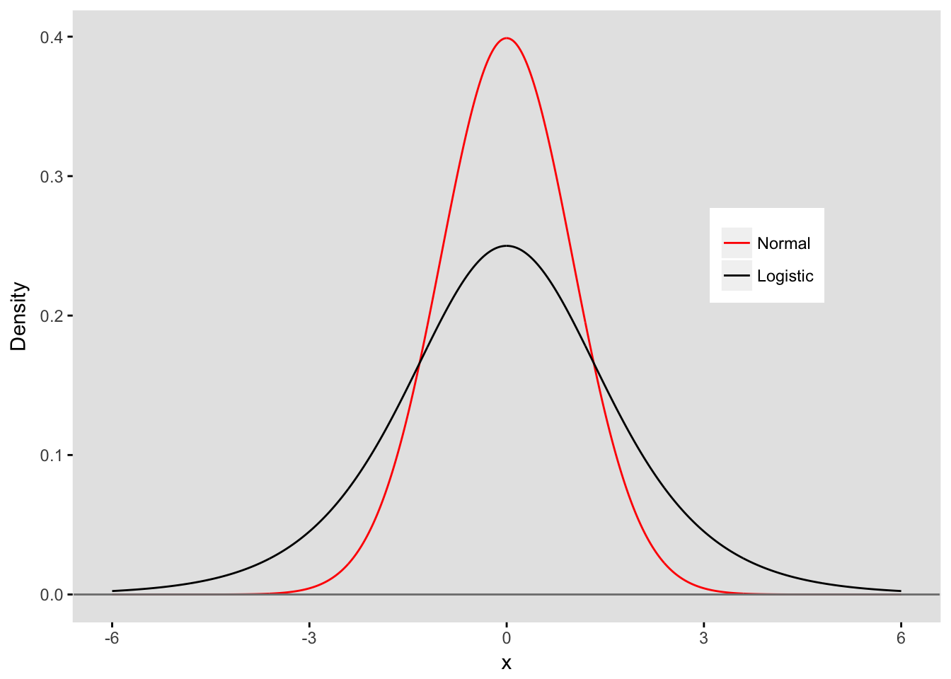
The threshold defines the probability
Below, I have plotted the standardized logistic pdf with a threshold that defines a tipping point for a particular Group A. In this case the threshold is 1.5, so for everyone with a unseen value of \(X < 1.5\), the observed binary outcome \(Y\) will be 1. For those where \(X \geq 1.5\), the observed binary outcome \(Y\) will be 0:
xGrpA <- 1.5

ggplot(data = dtm[variable == "yLogis"], aes(x = x, y = Density)) +
  geom_line() +
  geom_segment(x = xGrpA, y = 0, xend = xGrpA, yend = dlogis(xGrpA), lty = 2) +
  geom_area(mapping = aes(ifelse(x < xGrpA, x, xGrpA)), fill = "white") +
  geom_hline(yintercept = 0, color = "grey50") +
  ylim(0, 0.3) +
  my_theme() +
  scale_x_continuous(breaks = c(-6, -3, 0, xGrpA, 3, 6))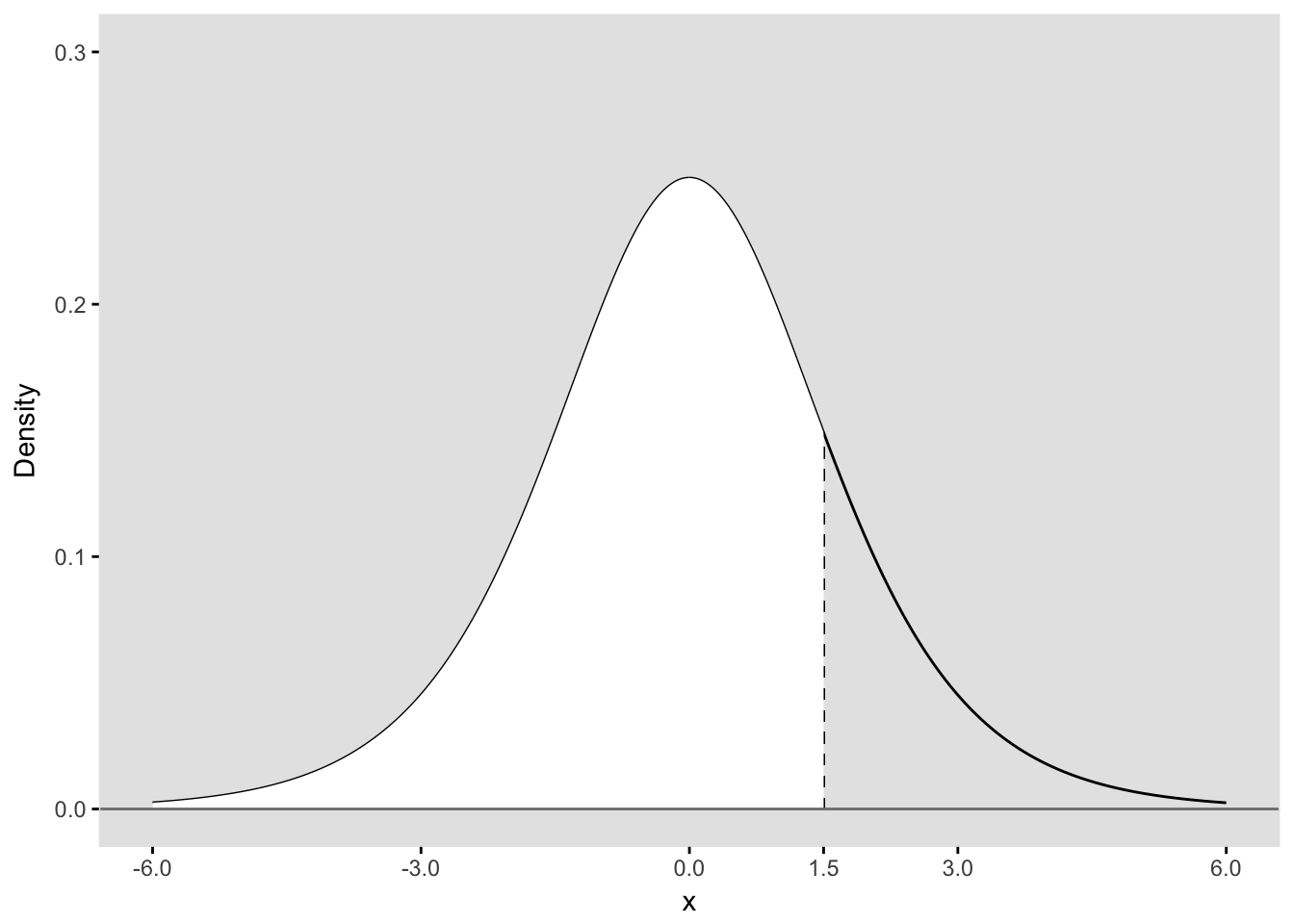
Since we have plot a probability density (pdf), the area under the entire curve is equal to 1. We are interested in the binary outcome \(Y\) defined by the threshold, so we can say that the area below the curve to the left of threshold (filled in white) represents \(P(Y = 1|Group=A)\). The remaining area represents \(P(Y = 0|Group=A)\). The area to the left of the threshold can be calculated in R using the plogis function:
(p_A <- plogis(xGrpA))## [1] 0.8175745Here is the plot for a second group that has a threshold of 2.2:
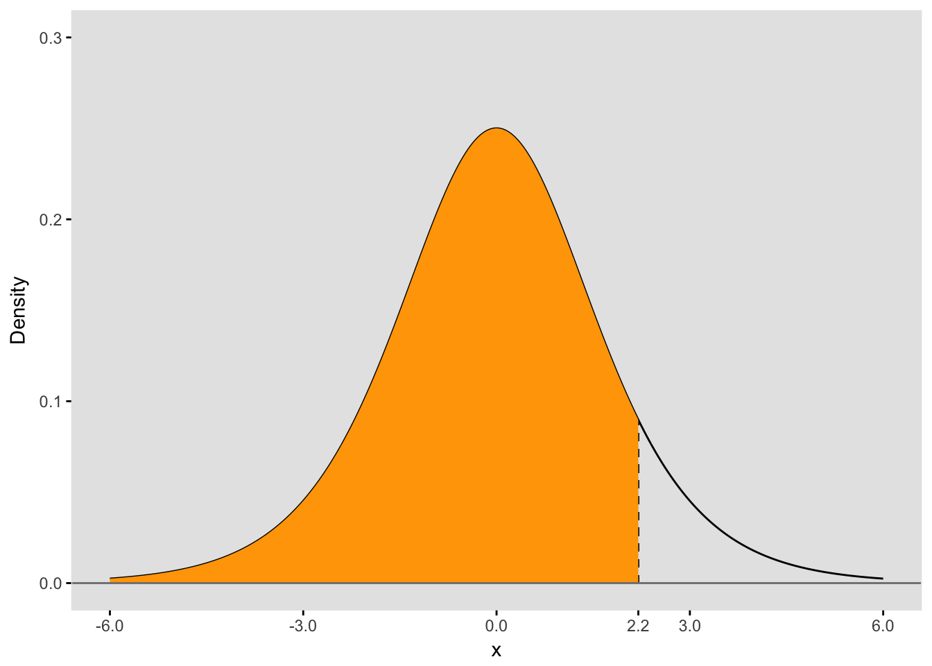
The area under the curve to the left of the threshold is \(P(X < 2.2)\), which is also \(P(Y = 1 | Group=B)\):
(p_B <- plogis(xGrpB))## [1] 0.9002495Log-odds and probability
In logistic regression, we are actually estimating the log-odds of an outcome, which can be written as
\[log \left[ \frac{P(Y=1)}{P(Y=0)} \right]\].
In the case of Group A, log-odds of Y being equal to 1 is
(logodds_A <- log(p_A / (1 - p_A) ))## [1] 1.5And for Group B,
(logodds_B <- log(p_B / (1 - p_B) ))## [1] 2.2As you may have noticed, we’ve recovered the thresholds that we used to define the probabilities for the two groups. The threshold is actually the log-odds for a particular group.
Logistic regression
The logistic regression model that estimates the log-odds for each group can be written as
\[log \left[ \frac{P(Y=1)}{P(Y=0)} \right] = B_0 + B_1 * I(Grp = B) \quad ,\]
where \(B_0\) represents the threshold for Group A and \(B_1\) represents the shift in the threshold for Group B. In our example, the threshold for Group B is 0.7 units (2.2 - 1.5) to the right of the threshold for Group A. If we generate data for both groups, our estimates for \(B_0\) and \(B_1\) should be close to 1.5 and 0.7, respectively
The process in action
To put this all together in a simulated data generating process, we can see the direct link with the logistic distribution, the binary outcomes, and an interpretation of estimates from a logistic model. The only stochastic part of this simulation is the generation of continuous outcomes from a logistic distribution. Everything else follows from the pre-defined group assignments and the group-specific thresholds:
n = 5000
set.seed(999)

# Stochastic step

xlatent <- rlogis(n, location = 0, scale = 1)

# Deterministic part

grp <- rep(c("A","B"), each = n / 2)

dt <- data.table(id = 1:n, grp, xlatent, y = 0)
dt[grp == "A" & xlatent <= xGrpA, y := 1]
dt[grp == "B" & xlatent <= xGrpB, y := 1]

# Look at the data

dt
## id grp xlatent y
## 1: 1 A -0.4512173 1
## 2: 2 A 0.3353507 1
## 3: 3 A -2.2579527 1
## 4: 4 A 1.7553890 0
## 5: 5 A 1.3054260 1
## ---
## 4996: 4996 B -0.2574943 1
## 4997: 4997 B -0.9928283 1
## 4998: 4998 B -0.7297179 1
## 4999: 4999 B -1.6430344 1
## 5000: 5000 B 3.1379593 0The probability of a “successful” outcome (i.e \(P(Y = 1\))) for each group based on this data generating process is pretty much equal to the areas under the respective densities to the left of threshold used to define success:
dt[, round(mean(y), 2), keyby = grp]## grp V1
## 1: A 0.82
## 2: B 0.90Now let’s estimate a logistic regression model:
library(broom)
glmfit <- glm(y ~ grp, data = dt, family = "binomial")
tidy(glmfit, quick = TRUE)
## term estimate
## 1 (Intercept) 1.5217770
## 2 grpB 0.6888526The estimates from the model recover the logistic distribution thresholds for each group. The Group A threshold is estimated to be 1.52 (the intercept) and the Group B threshold is estimated to be 2.21 (intercept + grpB parameter). These estimates can be interpreted as the log-odds of success for each group, but also as the threshold for the underlying continuous data generating process that determines the binary outcome \(Y\). And we can interpret the parameter for grpB in the traditional way as the log-odds ratio comparing the log-odds of success for Group B with the log-odds of success for Group A, or as the shift in the logistic threshold for Group A to the logistic threshold for Group B.
In the next week or so, I will extend this to a discussion of an ordinal categorical outcome. I think the idea of shifting the thresholds underscores the proportionality assumption I alluded to earlier …