simstudy 0.8.0: customized distributions

Specifying the customized distribution

When defining a custom distribution in defData, you provide the name of the user-defined function as a string in the formula argument. The arguments of this custom function are listed in the variance argument, separated by commas and formatted as “arg_1 = val_form_1, arg_2 = val_form_2, \(\dots\), arg_K = val_form_K”.

The arg_k’s represent the names of the arguments passed to the customized function, where \(k\) ranges from \(1\) to \(K\). You can use values or formulas for each val_form_k. If formulas are used, ensure that the variables have been previously generated. Double dot notation is available in specifying value_formula_k. It is important to note that the parameter list of the actual function must include an argument”n = n”, but \(n\) should not be included in the definition as part of defData or defDataAdd (specified in the variance field).

Example 1

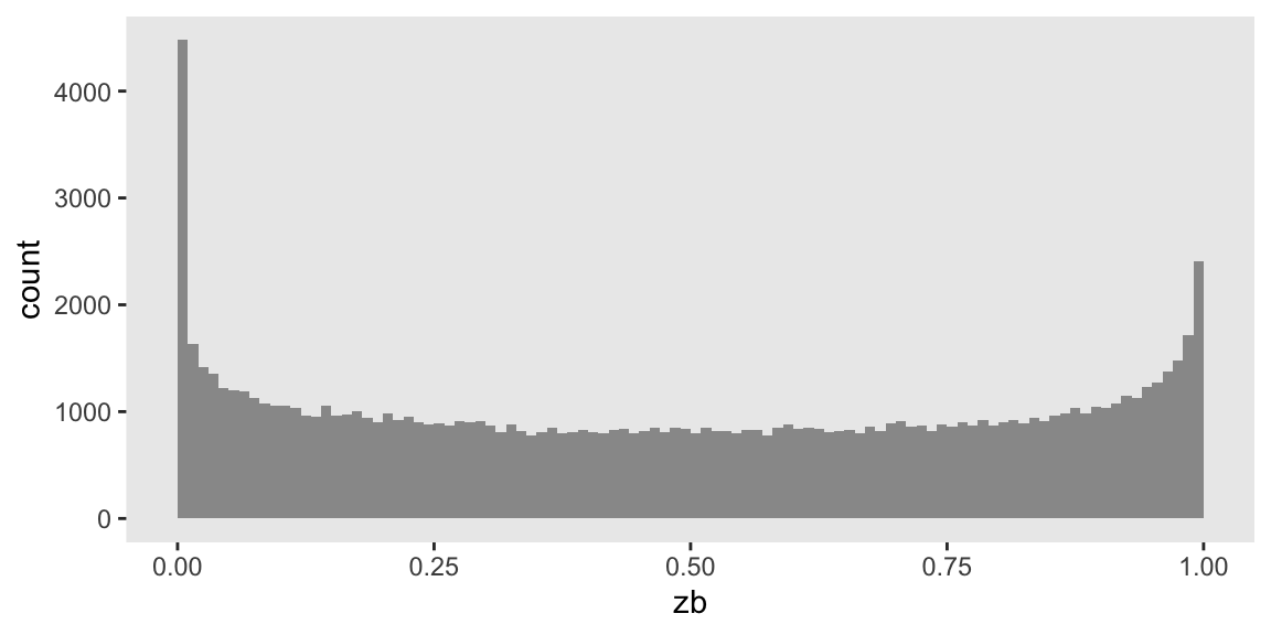
Here is an example where we generate data from a zero-inflated beta distribution. (I’ve implemented something like this in the past using a mixture distribution, which is also a fine way to go). I’ve created a user-defined function zeroBeta that takes on shape parameters \(a\) and \(b\) for the beta distribution, as well as \(p_0\), the proportion of the sample that takes on a value of zero. Note that the function also takes an argument \(n\) that will not to be be specified in the data definition; \(n\) will represent the number of observations being generated:

zeroBeta <- function(n, a, b, p0) {
  betas <- rbeta(n, a, b)
  is.zero <- rbinom(n, 1, p0)
  betas*!(is.zero)
}

The data definition specifies that we want to create a variable \(zb\) from the user-defined zeroBeta function with \(a\) and \(b\) set to 0.75, and \(p_0 = 0.02\):

def <- defData(
  varname = "zb", 
  formula = "zeroBeta", 
  variance = "a = 0.75, b = 0.75, p0 = 0.02", 
  dist = "custom"
)

The data are generated with a call to genData as is typically done in simstudy:

set.seed(1234)
dd <- genData(100000, def)

## Key: <id>
##             id         zb
##          <int>      <num>
##      1:      1 0.93922887
##      2:      2 0.35609519
##      3:      3 0.08087245
##      4:      4 0.99796758
##      5:      5 0.28481522
##     ---                  
##  99996:  99996 0.81740836
##  99997:  99997 0.98586333
##  99998:  99998 0.68770216
##  99999:  99999 0.45096868
## 100000: 100000 0.74101272

A plot of the data highlights an over-representation of zeroes:

Example 2

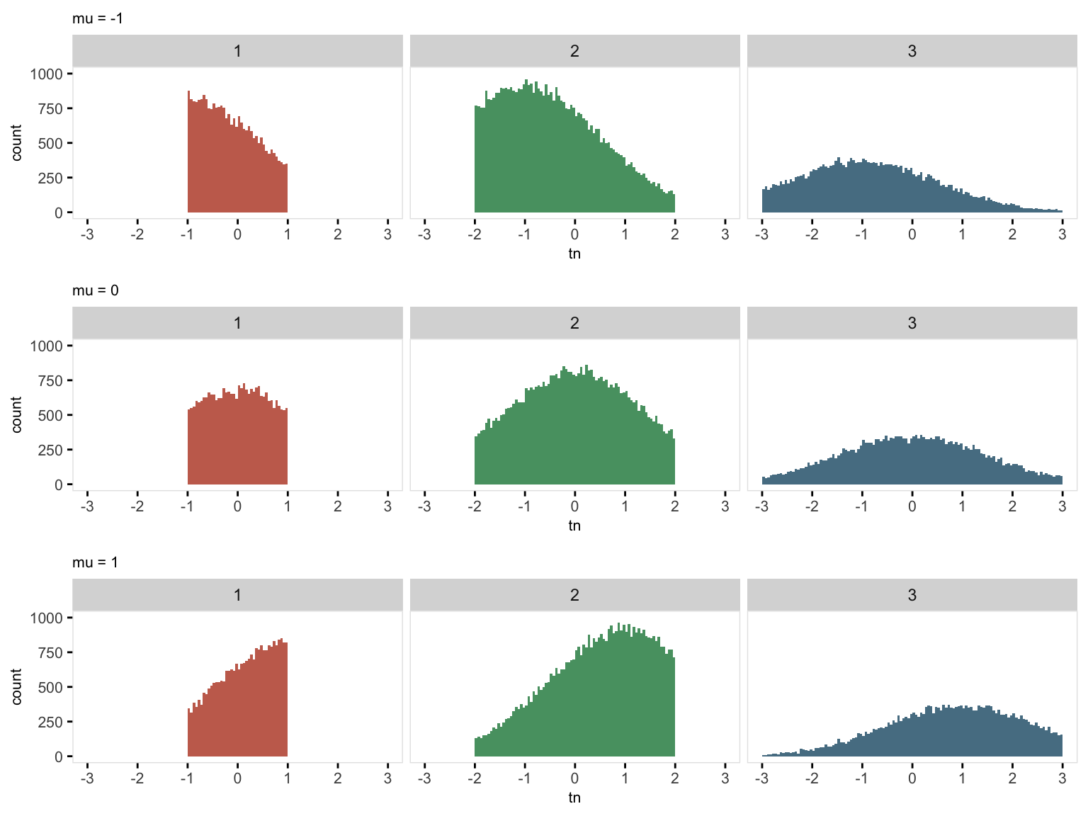
In this second example, I am generating sets of truncated Gaussian distributions with means ranging from \(-1\) to \(1\). (I wrote about this a while ago - the approach implemented here is an alternative way to generate these data.) rnormt is a customized (user-defined) function that generates the truncated Gaussian data, and requires four arguments (the left truncation value, the right truncation value, the distribution average without truncation and the distribution standard deviation without truncation):

rnormt <- function(n, min, max, mu, s) {
  
  F.a <- pnorm(min, mean = mu, sd = s)
  F.b <- pnorm(max, mean = mu, sd = s)
  
  u <- runif(n, min = F.a, max = F.b)
  qnorm(u, mean = mu, sd = s)
  
}

In this example, truncation limits differ based on group membership. Initially, three groups are created (represented by the variable defined as limit), followed by the generation of truncated values (named tn). For Group 1, truncation is defined by the range of \(-1\) to \(1\); for Group 2, the range is \(-2\) to \(2\); and for Group 3, the range is \(-3\) to \(3\). We’ll generate three data sets, each with a distinct mean denoted by M, using the double-dot notation to implement the different means.

def <-
  defData(
    varname = "limit", 
    formula = "1/4;1/2;1/4",
    dist = "categorical"
  ) |>
  defData(
    varname = "tn", 
    formula = "rnormt", 
    variance = "min = -limit, max = limit, mu = ..M, s = 1.5",
    dist = "custom"
  )

The data generation requires three calls to genData, one for each different mean value \(\mu\). I have chosen to implement this with lapply:

mu <- c(-1, 0, 1)
dd <-lapply(mu, function(M) genData(100000, def))

The output is a list of three data sets; here are the first six observations from each of the three data sets:

## [[1]]
## Key: <id>
##       id limit         tn
##    <int> <int>      <num>
## 1:     1     2  0.6949619
## 2:     2     2 -0.3641963
## 3:     3     2 -0.4721632
## 4:     4     3 -2.6083796
## 5:     5     2 -0.6800441
## 6:     6     3 -0.5813880
## 
## [[2]]
## Key: <id>
##       id limit         tn
##    <int> <int>      <num>
## 1:     1     1  0.4853614
## 2:     2     2 -0.5690811
## 3:     3     2  0.5282246
## 4:     4     2  0.1107778
## 5:     5     2 -0.3504309
## 6:     6     2  1.9439890
## 
## [[3]]
## Key: <id>
##       id limit         tn
##    <int> <int>      <num>
## 1:     1     2  1.3560628
## 2:     2     2  1.4543616
## 3:     3     3  1.4491010
## 4:     4     2  0.7328855
## 5:     5     2 -0.1254556
## 6:     6     2 -0.7455908

A plot highlights the group differences for each of the three data sets: