A three-arm trial using two-step randomization

Preliminaries

Before we get started, here are the libraries that will be need for the simulations, model fitting, and outputting the results:

library(simstudy)
library(ggplot2)
library(lmerTest)
library(data.table)
library(multcomp)
library(parallel)
library(flextable)

RNGkind("L'Ecuyer-CMRG")  # to set seed for parallel process

Three-arm cluster randomized trial

We’ll start with the three-arm cluster randomized trial, where providers would be randomized in a 1:1:1 ratio to either \(Control\), \(CDS\), or \(CDS+\). The data definitions for the cluster-level data includes a random effect \(b\) and a three-level treatment indicator \(A\). The individual-level outcome is a continuous variable centered around 0 for patients in the control arm (offset by the provider-specific random effect). The effect of CDS (compared to Control) is 1.5, and the incremental effect of CDS+ (compared to CDS) is 0.75.

defs <- 
  defData(varname = "b", formula = 0, variance = 1) |>
  defData(varname = "A", formula = "1;1;1", dist = "trtAssign") 

defy <- 
  defDataAdd(varname = "y", formula = "1.50 * (A==2) + 2.25 * (A==3) + b", variance = 8)

To generate a single data set, we generate the provider level data, add the patient-level records and generate the patient-level outcomes.

set.seed(9612)

dc <- genData(30, defs, id = "provider")
dd <- genCluster(dc, "provider", 40, "id")
dd <- addColumns(defy, dd)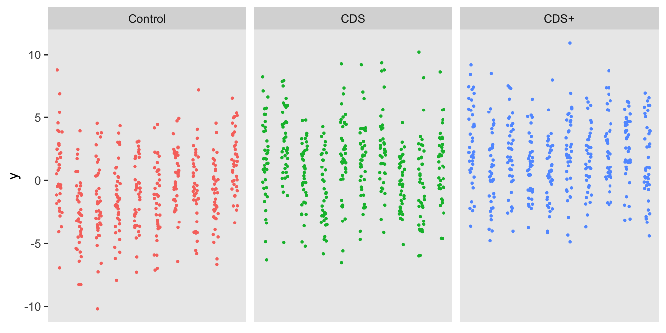

A mixed effects model with a provider-level random effect gives the parameter estimates for the effect of CDS (versus control) and CDS+ (also versus control):

lmerfit <- lmer(y ~ factor(A) + (1 | provider), data = dd)
as_flextable(lmerfit) |> delete_part(part = "footer")

However, we are really interested in comparing CDS with Control and CDS+ with CDS (and not CDS+ with control); we can use the glht package to provide the contrasts. To ensure that our overall Type I error rate is 5%, we use a Bonferroni-corrected p-value threshold of 0.025. In this particular case, we would not infer that there is any benefit to CDS+ over CDS, though it does appear that CDS is better than no CDS.

K1 <- matrix(c(0, 1, 0, 0, -1, 1), 2, byrow = T)
summary(glht(lmerfit, K1))

## 
## 	 Simultaneous Tests for General Linear Hypotheses
## 
## Fit: lmer(formula = y ~ factor(A) + (1 | provider), data = dd)
## 
## Linear Hypotheses:
##        Estimate Std. Error z value Pr(>|z|)    
## 1 == 0   1.8530     0.4794   3.865  0.00022 ***
## 2 == 0   0.7136     0.4794   1.488  0.23509    
## ---
## Signif. codes:  0 '***' 0.001 '**' 0.01 '*' 0.05 '.' 0.1 ' ' 1
## (Adjusted p values reported -- single-step method)

In the next step, I’m generating 2500 data sets and fitting a model for each one. The estimated parameters, standard errors, and p-values are saved to an R list so that I can estimate the power to detect an effect for each comparison (based on the assumptions used to generate the data):

genandfit <- function() {
  
  dc <- genData(30, defs, id = "provider")
  dd <- genCluster(dc, "provider", 40, "id")
  dd <- addColumns(defy, dd)
  
  lmerfit <- lmer(y ~ factor(A) + (1 | provider), data = dd)
  K1 <- matrix(c(0, 1, 0, 0, -1, 1), 2, byrow = T)
  data.table(ests = summary(glht(lmerfit, K1))$test$coefficients,
             sd = summary(glht(lmerfit, K1))$test$sigma,
             pvals = summary(glht(lmerfit, K1))$test$pvalues
  )
  
}

reps <- mclapply(1:2500, function(x) genandfit())
reps[1:3]

## [[1]]
##         ests        sd       pvals
## 1: 1.6634678 0.5213168 0.002768887
## 2: 0.8372875 0.5213168 0.189092375
## 
## [[2]]
##         ests        sd        pvals
## 1: 0.8206728 0.4380257 0.1097610533
## 2: 1.6465060 0.4380257 0.0003375337
## 
## [[3]]
##        ests        sd        pvals
## 1: 1.340631 0.4691332 0.0082278928
## 2: 1.777505 0.4691332 0.0002994282

The estimated power for each effect estimate is the proportion of iterations with a p-value less than 0.025. Using this standard cluster-randomized three-arm study design, there is 74% power to detect a difference between CDS and Control when the true difference is 1.50, and only 19% power to detect a difference between CDS+ and CDS when the true difference is 0.75:

pvals <- rbindlist(mclapply(reps, function(x) data.table(t(x[, pvals]))))
pvals[, .(`CDS vs Control` = mean(V1 < 0.025), `CDS+ vs CDS` = mean(V2 < 0.025))]

##    CDS vs Control CDS+ vs CDS
## 1:         0.7356      0.1904

Two-step randomization

The same process can be applied to evaluate the two-step randomization. In this formulation, the clusters are randomized in a 1:2 ratio to control \((A = 0)\) or CDS \((A = 1)\). For the the clusters randomized to CDS (\(2/3\) of the total clusters), the individual patients are randomized to standard CDS \((X=0)\) or CDS+ \((X=1)\). The randomization is stratified by provider with a 1:1 ratio. The randomization scheme is facilitated by the simstudy defCondition and addCondition functions. For the patients in the control arm, \(A=0\) and \(X=0\).

The individual outcome \(y\) is generated slightly differently than in the three-arm trial, but the effect sizes are equivalent: 1.50 point difference between standard CDS and control and 0.75 difference between CDS+ and CDS.

defs <- 
  defData(varname = "b", formula = 0, variance = 1) |>
  defData(varname = "A", formula = "1;2", dist = "trtAssign")

defc <- 
  defCondition(condition = "A == 1", formula = "1;1", 
    variance = "provider", dist = "trtAssign") |>
  defCondition(condition = "A == 0", formula = 0, 
    dist = "nonrandom")

defy <- 
  defDataAdd(varname = "y", formula = "1.50 * A + 0.75 * X + b", variance = 8)

dc <- genData(30, defs, id = "provider")
dd <- genCluster(dc, "provider", 40, "id")
dd <- addCondition(defc, dd, "X")
dd <- addColumns(defy, dd)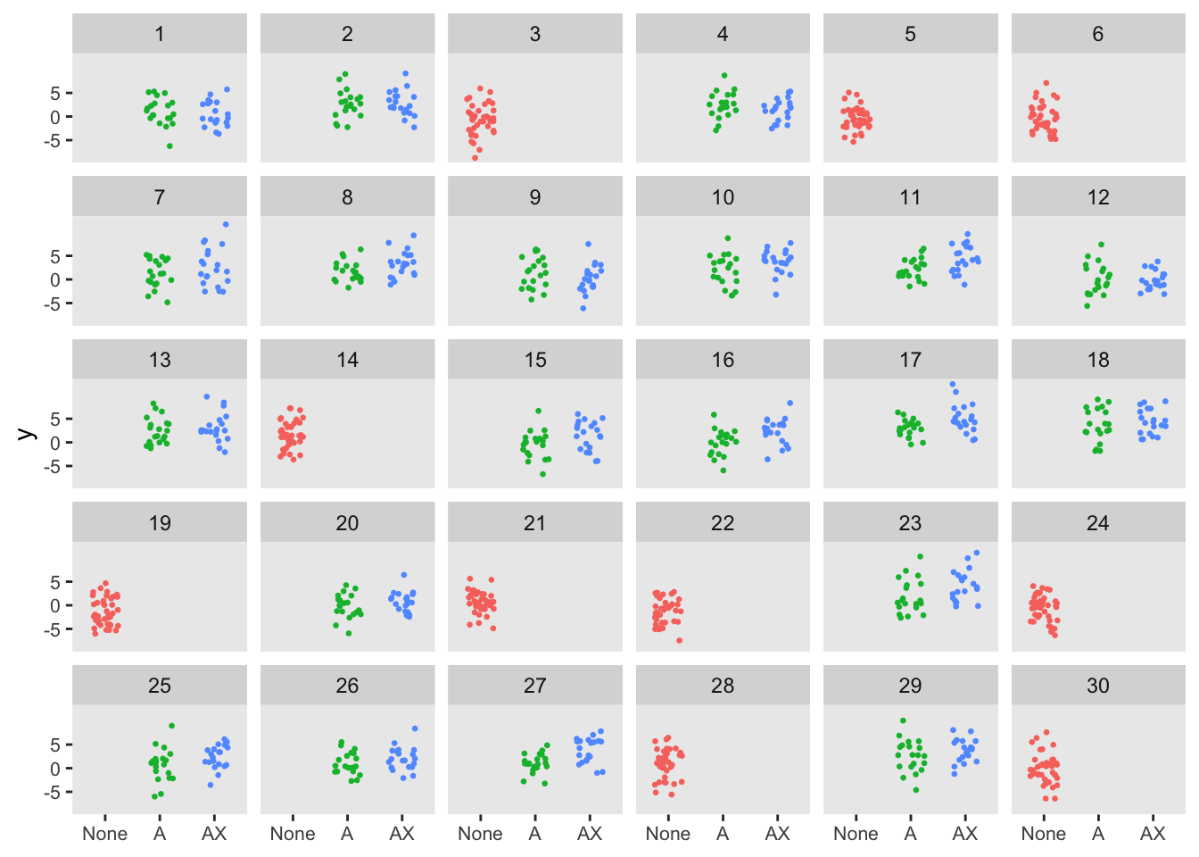

The model for this data set also looks slightly different than the three arm case, as we can model the CDS+ vs CDS directly; as a result, there is no need to consider the contrasts. In this example, we would conclude that CDS+ is an improvement over CDS and CDS is better than no CDS.

lmerfit <- lmer(y ~ A + X + (1|provider), data = dd)
as_flextable(lmerfit) |> delete_part(part = "footer")

The estimated the power from replicated data sets makes it pretty clear that the two-step randomization design has considerably more power for both effects, each reaching the 80% threshold.

pvals[, .(`CDS vs Control` = mean(A < .025), `CDS+ vs CDS` = mean(X < 0.025))]

##    CDS vs Control CDS+ vs CDS
## 1:         0.8392      0.8544

While it appears that the two-step randomization design is clearly superior to the three-arm cluster randomized design, it is important to again point out the key caveat here that, conditional on the provider, the patient outcomes in the CDS and CDS+ arms patients need to be independent of each other. For example, if the provider can’t avoid applying CDS+ tools to the CDS only patients, this assumption of independence is violated and the two-step design is not going to be appropriate. Instead, a three-arm cluster randomized design with more providers (clusters) will be needed.