Over the past couple of years, I have been working with an amazing group of investigators as part of the CONTAIN trial to study whether COVID-19 convalescent plasma (CCP) can improve the clinical status of patients hospitalized with COVID-19 and requiring noninvasive supplemental oxygen. This was a multi-site study in the US that randomized 941 patients to either CCP or a saline solution placebo. The overall findings suggest that CCP did not benefit the patients who received it, but if you drill down a little deeper, the story may be more complicated than that.
Of course, it is the “drilling down” part that gets people (and biostatisticians) a little nervous. Once we get beyond the primary analysis, all bets are off. If we look hard enough at the data, we may eventually find something that is interesting to report on. But, just because we find something with the data in hand, it does not mean that we would find it again in another data set from another study. Any conclusions we draw may be unwarranted:

Source: XKCD
The CONTAIN trial was conducted under very difficult circumstances, where the context was rapidly changing over time. Particularly challenging was the fact that new therapies were introduced for hospitalized patients over the course of the trial. And when we looked at the data, we noticed that while all patients had poor clinical outcomes in the first several months of the study, CCP appeared to offer some benefits. Later on in the study, when corticosteroids and remdesivir were standard of care, overall patient outcomes were dramatically improved, and CCP was no longer providing any benefits. This was a very interesting finding that we felt merited some discussion.
Not surprisingly, we have received some push back, suggesting that this finding is a classic case of regression to the mean. Normally, I would not have been comfortable presenting those findings, particularly not in a highly visible journal article. But we had used a Bayesian modelling framework with quite quite skeptical prior distribution assumptions to evaluate the primary outcome and the exploratory outcomes, so we felt that while we needed to be cautious in how we presented the results, these were not green jelly bean findings. Given the strong biological plausibility, we felt quite strongly about adding these findings to the growing body of literature about CCP.
In this post, I am sharing a series of simulations to explore how conservative our conservative approach really is. This is another look at assessing Type I error rates, a frequentist notion, in the context of a Bayesian study design.
The subgroup-specific treatment effect
Let’s say there is a data generation process for individual \(i\) with a (binary) outcome \(Y_i\) with some (binary) treatment or exposure \(A_i\) that looks like
\[log\left(\frac{P(Y_i=1)}{P(Y_i=0)}\right ) = \alpha + \delta A_i.\]
The log-odds is dependent only on the level of exposure \(A\).
Let’s say that we’ve also measured some characteristic \(G\), which is a categorical variable with three levels. While the primary aim of the study is to estimate \(\delta\), the log-odds ratio comparing treated with controls, we might also be interested in a subgroup analysis based on \(G\). That is, is there a unique group-level treatment effect for any level of \(G\), \(G \in \{1,2,3\}\)? In terms of the model, this would be
\[ log\left(\frac{P(Y_i=1|G_i=g)}{P(Y_i=0|G_i=g)}\right ) = \alpha_g + \delta_g A_i, \ \ g \in \{1,2,3\}.\]
In the case here, we actually know that \(\alpha_g = \alpha\) and \(\delta_g = \delta\) for all \(g\) because the data generation process is independent of \(G\). However, due to sampling error it is quite possible that we will observe some differences in the data.
Simulation
We start by simulating this case of a single grouping with three potential subgroup analyses. First, here are the libraries used to create the examples in this post:
library(simstudy)
library(data.table)
library(posterior)
library(bayesplot)
library(cmdstanr)
library(gtsummary)
library(paletteer)
library(ggplot2)
library(ggdist)
Data generation
I’m generating 1000 subjects, with 500 in each treatment arm \(A\). About a third fall into each level of \(G\), and the binary outcome \(Y\) takes a value of \(1\) \(10\%\) of the time for all subjects regardless of their treatment or group level
def <- defData(varname = "g", formula = "1/3;1/3;1/3", dist = "categorical")
def <- defData(def, "a", formula = "1;1", dist = "trtAssign")
def <- defData(def, "y", formula = "0.10", dist = "binary")

RNGkind("L'Ecuyer-CMRG")
set.seed(67)

dd <- genData(1000, def)
dd
## id g a y
## 1: 1 3 1 0
## 2: 2 3 1 0
## 3: 3 2 1 0
## 4: 4 2 0 0
## 5: 5 3 0 0
## ---
## 996: 996 2 0 0
## 997: 997 1 0 0
## 998: 998 1 1 0
## 999: 999 3 0 0
## 1000: 1000 3 1 0We can fit a simple logistic regression model to estimate \(\delta\), the overall effect of the treatment. We see that the estimate of the OR is very close to 1, suggesting the odds of \(Y=1\) is similar for both groups, so no apparent treatment effect. (Note that the exponentiated intercept is an estimate of the odds of \(Y=1\) for the control arm. The data generation process assumed \(P(Y=1) = 0.10\), so the odds are \(0.1/0.9 = 0.11\).)
fitglm <- glm(y ~ a, data = dd, family = "binomial")
tbl_regression(fitglm, intercept = TRUE, exponentiate = TRUE)| Characteristic | OR1 | 95% CI1 | p-value |
|---|---|---|---|
| (Intercept) | 0.11 | 0.08, 0.14 | <0.001 |
| a | 1.02 | 0.67, 1.55 | >0.9 |
|
1
OR = Odds Ratio, CI = Confidence Interval
|
|||
So, we could not infer that for the entire group treatment \(A\) has any effect. But, maybe for some subgroups there is a treatment effect? We can fit a generalized linear model that allows the intercept and effect estimate to vary by level of \(G\), and assess whether this is the case for subgroups defined by \(G\).
fitglm <- glm(y ~ factor(g) + a:factor(g) - 1, data = dd, family = "binomial")
tbl_regression(fitglm, exponentiate = TRUE)| Characteristic | OR1 | 95% CI1 | p-value |
|---|---|---|---|
| factor(g) | |||
| 1 | 0.09 | 0.05, 0.15 | <0.001 |
| 2 | 0.11 | 0.07, 0.18 | <0.001 |
| 3 | 0.12 | 0.08, 0.20 | <0.001 |
| factor(g) * a | |||
| 1 * a | 1.23 | 0.57, 2.76 | 0.6 |
| 2 * a | 1.24 | 0.64, 2.45 | 0.5 |
| 3 * a | 0.69 | 0.32, 1.44 | 0.3 |
|
1
OR = Odds Ratio, CI = Confidence Interval
|
|||
While there is more variability in the estimates, we still wouldn’t conclude that there are treatment effects within each level of \(G\).
The Bayesian model
Since the purpose of this post is to illustrate how an appropriately specified Bayesian model can provide slightly more reliable estimates, particularly in the case where there really are no underlying treatment effects, here is a Bayes model that estimates subgroup-level intercepts and treatment effects:
\[Y_{ig} \sim Bin(p_{ig})\] \[log\left(\frac{p_{ig}}{1-p_{ig}}\right) = \alpha_g + \delta_gA_i, \ \ g \in \{1,2,3\} \]
The prior distribution assumptions for the parameters \(\alpha_g\) and \(\delta_g\) are
\[\begin{aligned} \alpha_g &\sim N(\mu = 0, \sigma = 10), \ \ g \in \{1,2,3\} \\ \delta_g &\sim N(\mu=\delta, \sigma = 0.3537), \ \ g \in \{1,2,3\} \\ \delta &\sim N(\mu = 0, \sigma = 0.3537) \end{aligned}\]Note that the variance of the \(\delta_g\text{'s}\) around \(\delta\) has been specified, but it could be estimated. However, since there are very few levels of \(G\), estimation of the variance can be slow; to speed the simulations, I’ve chosen a quicker path by specifying a pretty informative prior.
Fitting the Bayes model
The Stan code that implements this model can be found in the addendum. To estimate the model, the the data need to be passed as a list - and here is a function to convert the R data into the proper format:
listdat <- function(dx, grpvar) {

  dx[, grp := factor(get(grpvar))]

  N <- dx[, .N]
  L <- dx[, nlevels(grp)]
  y <- dx[, y]
  a <- dx[, a]
  grp <-dx[, as.numeric(grp)]

  list(N = N, L = L, y = y, a = a, grp = grp)
}
After compiling the program, samples from the posterior are drawn using four chains. There will be a total of 12000 samples (not including the warm-up samples):
mod <- cmdstan_model("extra/simulation.stan")

fitbayes <- mod$sample(
    data = listdat(dd, "g"),
    refresh = 0,
    chains = 4L,
    parallel_chains = 4L,
    iter_warmup = 1500,
    iter_sampling = 3000
)
## Running MCMC with 4 parallel chains...
##
## Chain 3 finished in 5.3 seconds.
## Chain 2 finished in 5.7 seconds.
## Chain 1 finished in 5.9 seconds.
## Chain 4 finished in 6.1 seconds.
##
## All 4 chains finished successfully.
## Mean chain execution time: 5.8 seconds.
## Total execution time: 6.2 seconds.The estimates are quite similar to the glm estimates, though the ORs are pulled slightly towards 1 as a result of the informative prior. This is going to be the trick that ultimately protects the Type I error rate from completely blowing up.
fitbayes$summary(c("Odds_g","OR_g"))## # A tibble: 6 × 10
## variable mean median sd mad q5 q95 rhat ess_bulk ess_tail
## <chr> <dbl> <dbl> <dbl> <dbl> <dbl> <dbl> <dbl> <dbl> <dbl>
## 1 Odds_g[1] 0.0932 0.0910 0.0237 0.0230 0.0586 0.136 1.00 8636. 9489.
## 2 Odds_g[2] 0.118 0.116 0.0258 0.0254 0.0800 0.165 1.00 8924. 8875.
## 3 Odds_g[3] 0.115 0.112 0.0262 0.0260 0.0757 0.161 1.00 9734. 9569.
## 4 OR_g[1] 1.16 1.11 0.345 0.317 0.689 1.80 1.00 8077. 8824.
## 5 OR_g[2] 1.17 1.13 0.320 0.300 0.724 1.77 1.00 7922. 8641.
## 6 OR_g[3] 0.884 0.848 0.256 0.239 0.527 1.36 1.00 8817. 8620.And here is a plot of the posterior distributions for the treatment effect at each subgroup defined by the levels of \(G\):
OR_df <- data.frame(as_draws_rvars(fitbayes$draws(variables = "OR_g")))

p_data <- with(OR_df, data.frame(
  cat = c("c1", "c2", "c3"),
  OR_g = OR_g
))

ggplot(data = p_data, aes(dist = OR_g, y = cat)) +
  geom_vline(xintercept = 1, color = "grey80", size = .3) +
  stat_dist_halfeye(fill = palettes_d$awtools$a_palette[6], position="dodge") +
  theme(panel.grid = element_blank()) +
  ylab("category") +
  scale_x_continuous(limits = c(0, 2), name = "OR")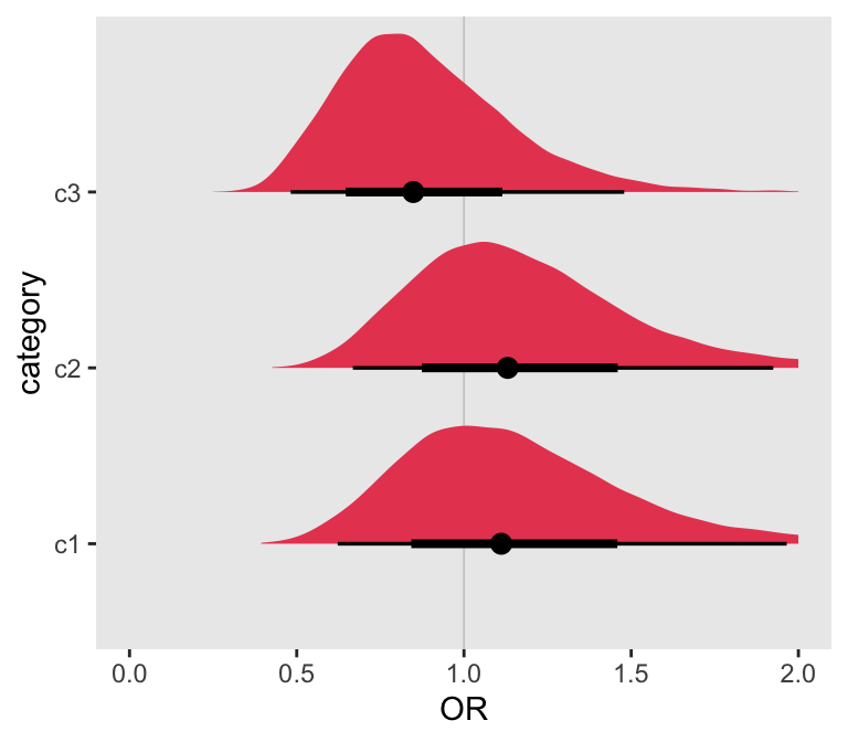
It is easy to see that the 95% credible intervals all include the value of 1, no treatment effect, so we wouldn’t be tempted to conclude that there is any treatment effect. We can also check manually to see if at least one of the credible intervals excludes 1. The answer is still “no.”
with(OR_df, any((quantile(OR_g, .025) > 1) | (quantile(OR_g, .975) < 1)))## [1] FALSEIncreasing the number of subgroups
As the jelly beans make clear, things can really start to go awry when we start to investigate many possible subgroups. This can either be a single characteristic (like color) that has many, many levels, each of which can be a subgroup, or this can be many different characteristics that each have a few different levels. In our trial, we had the latter, all based on baseline data collection (and all reported as categories). These included health status, age, blood type, time between COVID symptom onset, medications, quarter of enrollment, and others.
My interest here is to see how fast the Type I error increases as the number of subgroups increases. I consider that a Type I error has occurred if any of the subgroups would be declared what I am calling potentially “interesting”. “Interesting” and by no means definitive, because while the results might suggest that treatment effects are stronger in a particular subgroup, we do need to be aware that these are exploratory analyses.
To explore Type I error rates, I will generate 20 categories, each of which has three levels. I can then use the model estimates from each of the subgroup analyses to evaluate how many times I would draw the wrong conclusion.
Generating multiple categories
To illustrate how I code all of this, I am starting with a case where there are four categories, each with three levels. In the data set, these categories are named g1, g2, g3, and g4:
genRepeatDef <- function(nvars, prefix, formula, variance, dist, link = "identity") {
  varnames <- paste0(prefix, 1 : nvars)
  data.table(varname = varnames,
             formula = formula,
             variance = variance,
             dist = dist, link = link)
}

def <- genRepeatDef(4, "g", "1/3;1/3;1/3", 0, "categorical")
def <- defData(def, "a", formula = "1;1", dist = "trtAssign")
def <- defData(def, "y", formula = "0.10", dist = "binary")

def
## varname formula variance dist link
## 1: g1 1/3;1/3;1/3 0 categorical identity
## 2: g2 1/3;1/3;1/3 0 categorical identity
## 3: g3 1/3;1/3;1/3 0 categorical identity
## 4: g4 1/3;1/3;1/3 0 categorical identity
## 5: a 1;1 0 trtAssign identity
## 6: y 0.10 0 binary identityA single data set based on these definitions looks like this:
RNGkind("L'Ecuyer-CMRG")
set.seed(67) #4386212 83861 7611291

dd <- genData(1000, def)
dd
## id g1 g2 g3 g4 a y
## 1: 1 3 3 2 1 0 0
## 2: 2 3 3 1 3 1 1
## 3: 3 2 3 2 1 1 0
## 4: 4 2 1 1 1 0 0
## 5: 5 3 1 2 3 0 0
## ---
## 996: 996 2 1 2 1 0 0
## 997: 997 1 1 2 2 1 0
## 998: 998 1 1 2 1 0 0
## 999: 999 3 2 1 1 1 0
## 1000: 1000 3 3 3 3 1 0The function fitmods estimates both the glm and stan models for a single category. The models provide subgroup estimates of treatment effects, just as the example above did:
fitmods <-function(dx, grpvar) {

  # GLM

  dx[, grp := factor(get(grpvar))]
  fitglm <- glm(y ~ grp + a:grp - 1, data = dx, family = "binomial")

  pvals <- coef(summary(fitglm))[, "Pr(>|z|)"]

  lpval <- length(pvals)
  freq_res <- any(pvals[(lpval/2 + 1) : lpval] < 0.05)

  # Bayes

  dat <- listdat(dx, grpvar)

  fitbayes <- mod$sample(
    data = dat,
    refresh = 0,
    chains = 4L,
    parallel_chains = 4L,
    iter_warmup = 1500,
    iter_sampling = 3000
  )

  OR_df <- data.frame(as_draws_rvars(fitbayes$draws(variables = "OR_g")))
  bayes_res <- with(OR_df,
    any((quantile(OR_g, .025) > 1) | (quantile(OR_g, .975) < 1)))

  # Return results

  list(type1_dt = data.table(var = grpvar, bayes_res, freq_res),
       OR_post = data.frame(var = grpvar, cat = paste0("c",1:3), OR_df)
  )

}
In this case, I am calling the function fitmods for each of the four categorical groupings g1 through g4:
res <- lapply(paste0("g", 1:4), function(a) fitmods(dd, a))## Running MCMC with 4 parallel chains...
##
## Chain 2 finished in 5.3 seconds.
## Chain 1 finished in 5.4 seconds.
## Chain 4 finished in 5.5 seconds.
## Chain 3 finished in 5.7 seconds.
##
## All 4 chains finished successfully.
## Mean chain execution time: 5.5 seconds.
## Total execution time: 5.7 seconds.
## Running MCMC with 4 parallel chains...
##
## Chain 2 finished in 5.5 seconds.
## Chain 1 finished in 5.6 seconds.
## Chain 3 finished in 5.6 seconds.
## Chain 4 finished in 5.5 seconds.
##
## All 4 chains finished successfully.
## Mean chain execution time: 5.5 seconds.
## Total execution time: 5.6 seconds.
## Running MCMC with 4 parallel chains...
##
## Chain 4 finished in 5.5 seconds.
## Chain 2 finished in 5.6 seconds.
## Chain 1 finished in 5.8 seconds.
## Chain 3 finished in 5.9 seconds.
##
## All 4 chains finished successfully.
## Mean chain execution time: 5.7 seconds.
## Total execution time: 5.9 seconds.
## Running MCMC with 4 parallel chains...
##
## Chain 2 finished in 5.8 seconds.
## Chain 1 finished in 5.8 seconds.
## Chain 3 finished in 5.8 seconds.
## Chain 4 finished in 6.0 seconds.
##
## All 4 chains finished successfully.
## Mean chain execution time: 5.9 seconds.
## Total execution time: 6.1 seconds.One of the arguments returned by fitmods is a data.table of summary results for each of the four categorical grouping. If any of the effect estimates for one or more of the three subgroup levels in a category was deemed “interesting” (based on a p-value < 0.05 for the glm model, and the value 1 falling outside the 95% credible interval for the stan model), then the function returned a value of 1 or TRUE. In this case, at least one of the subgroups within g4 would have been declared interesting based on the glm and stan models; at least one of the subgroups within g2 would have been deemed interesting, but only based on the glm model:
type1_dt <- rbindlist(lapply(res, function(x) x$type1_dt))
type1_dt
## var bayes_res freq_res
## 1: g1 FALSE FALSE
## 2: g2 FALSE TRUE
## 3: g3 FALSE FALSE
## 4: g4 TRUE TRUEWe can see this visually for the stan models by looking at the density plots for each subgroup within each category:
dc <- do.call("rbind", lapply(res, function(x) x$OR_post))

ggplot(data = dc, aes(dist = OR_g, y = cat)) +
  geom_vline(xintercept = 1, color = "grey80", size = .3) +
  stat_dist_halfeye(fill = palettes_d$awtools$a_palette[7], alpha = .8) +
  theme(panel.grid = element_blank()) +
  xlab("OR") +
  facet_wrap(~ var)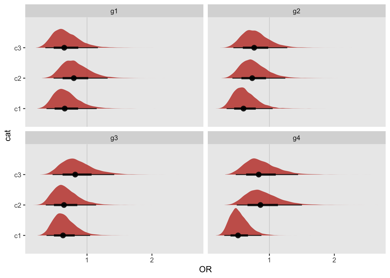
We calculate the first occurrence of an interesting subgroup by looking across g1 through g4. This will be useful for figuring out the Type I error rates for different numbers of categories. In this case, the first interesting subgroup based on the stan model is found when there are four categories; for the glm model, the first interesting subgroup is with two categories.
first_true <- sapply(type1_dt[, c(2,3)], function(x) match(TRUE, x))
first_true
## bayes_res freq_res
## 4 2Simulation study results
Now, with that background, here are the results based on 1050 simulated data sets (because I had access to 75 cores on a high performance computing cluster) with 20 categorical groups of three levels each. For each data set \(r, \ r \in \{1,\dots,1050\}\), I determined the first occurrence of an “interesting” finding among the 20 categories for each model, and stored this in \(F_{br}\) and \(F_{fr}\) for the Bayes and frequentist models, respectively. \(T_m(g)\) is the error rate for the model type \(m\), \(m \in \{b, f\}\) with \(g\) number of categories, and
\[ T_m(g) = \frac{\sum_{r=1}^{1050} I(F_{mr} \le g)}{1050} \]
Here is a plot of the Type I error rates calculated different numbers of categories. With the frequentist model (based on p-values) the error rates get quite large quite quickly, exceeding 50% by the time we reach 8 categories. In comparison, the error rates under the Bayes model with skeptical prior assumptions are held in check quite a bit better.
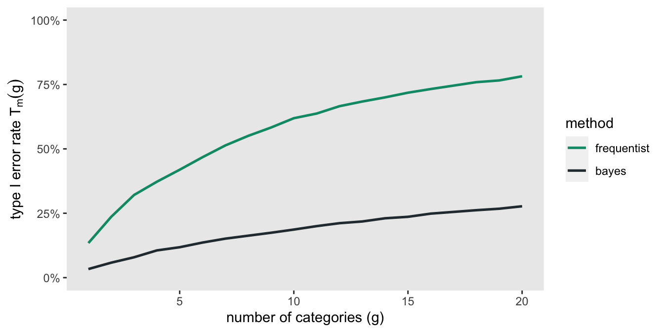
Even for the Bayes approach, however, the error rate is close to 20% for 12 categories. So, we still need to be careful in drawing conclusions. In the case that we do find some potentially interesting results (which we did in the case of the CCP CONTAIN trial), readers certainly have a right to be skeptical, but there is no reason to completely dismiss the findings out of hand. These sorts of findings suggest that more work needs to be done to better understand the nature of the treatment effects.
Addendum
data {
  int<lower=0> N;              // number of observations
  int<lower=1> L;              // number of levels
  int<lower=0,upper=1> y[N];   // vector of categorical outcomes
  int<lower=0,upper=1> a[N];   // treatment arm for individual
  int<lower=1,upper=4> grp[N]; // grp for individual
}

parameters {
  vector[L] alpha_g;           // group effect
  real delta_g[L];             // group treatment effects
  real delta;                  // overall treatment effect
}

transformed parameters{

  vector[N] yhat;

  for (i in 1:N)
    yhat[i] = alpha_g[grp[i]] + a[i] * delta_g[grp[i]];
}

model {

  // priors

  alpha_g ~ normal(0, 10);
  delta_g ~ normal(delta, 0.3537);
  delta ~ normal(0, 0.3537);

  // outcome model

  for (i in 1:N)
    y[i] ~  bernoulli_logit(yhat[i]);
}

generated quantities {

  real<lower = 0> OR_g[L];
  real<lower = 0> Odds_g[L];

  real<lower = 0> OR;

  for (i in 1:L) {
    OR_g[i] = exp(delta_g[i]);
    Odds_g[i] = exp(alpha_g[i]);
  }

  OR = exp(delta);

}