Recently, a colleague submitted a paper describing the results of a Bayesian adaptive trial where the research team estimated the probability of effectiveness at various points during the trial. This trial was designed to stop as soon as the probability of effectiveness exceeded a pre-specified threshold. The journal rejected the paper on the grounds that these repeated interim looks inflated the Type I error rate, and increased the chances that any conclusions drawn from the study could have been misleading. Was this a reasonable position for the journal editors to take?
My colleague’s experience resonated with me, as I’ve been thinking a bit about how frequentist concepts like Type I error rates and statistical power should be considered in the context of studies that are using Bayesian designs and modeling. Although these frequentist probabilities are not necessarily a natural logical or philosophical fit with the Bayesian approach, many reviewers, funders, and regulators will often require that the Bayesian design be justified by confirming control of Type I error at a pre-specified level.
My first inclination, of course, was to do a quick simulation to see if the journal’s concerns had any merit. So, I generated lots of data sets with two treatment arms but no treatment effect and simulated interim looks for each data set; my goal was to see how frequently we would be misled by the findings to draw unwarranted conclusions. Spoiler alert: the editor had reasons to be concerned; however, if we make some modifications to the evaluation criteria, we may be able to alleviate some of those concerns. This post documents the process and shows some results.
A little philosophy
Any post describing Bayesian models, p-values, and Type I errors - even one focused on simulation - would be remiss without at least some discussion of underlying philosophical differences between the two approaches. To start, this statement succinctly describes a key conflict:
The Bayesian approach is based on determining the probability of a hypothesis with a model using an “a priori” probability that is then updated based on data. On the contrary, [in] classical hypothesis testing … the error-I type is the probability of wrongly refusing the null hypothesis when it is true. Thus, [frequentist logic] is completely different from Bayesian logic (since probability is referred to making a mistake, not to the hypothesis itself).
So, the Bayesian approach is concerned with estimating \(P(hypothesis \ | \ data)\), whereas the frequentist p-value is an estimate of \(P(data \ | \ null \ hypothesis)\), quite different animals and it isn’t obvious they can be reconciled. Indeed, as Frank Harrell points out, there is a logical inconsistency with assuming that a particular (null) hypothesis is true and then trying to draw conclusions about that very same hypothesis:
The probability of a treatment not being effective is the probability of ``regulator’s regret.’’ One must be very clear on what is conditioned upon (assumed) in computing this probability. Does one condition on the true effectiveness or does one condition on the available data? Type I error conditions on the treatment having no effect … Can one quantify evidence for making a wrong decision if one assumes that all conclusions of non-zero effect are wrong up front because \(H_0\) was assumed to be true? Aren’t useful error probabilities the ones that are not based on assumptions about what we are assessing but rather just on the data available to us? [emphasis added]
In addition to Harrell’s post, there is a paper by Greenland et al that describes how statistical tests, confidence intervals, and statistical power can easily be misinterpreted and abused. However, these points of view have not been fully adopted by the scientific community more broadly, and Type I error rates and statistical power are still the predominant way of evaluating study designs.
This paper by Ryan et al acknowledges these realities while asking whether “we need to adjust for interim analyses in a Bayesian adaptive trial design?” The conclusion is “yes” if the goal is indeed to satisfy operating characteristics defined within the frequentist paradigm - and I will get to that in a second - but they conclude, maybe a little wistfully, that
if we avoid this dichotomisation [reject or fail to reject] and simply report the posterior probability of benefit, then we could potentially avoid having to specify the type I error of a Bayesian design.
But until more reviewers and funders accept this, investigators who opt for a Bayesian approach will likely still be required to square this circle.
Simulating interim looks
To assess the Type I error, I’ve used a relatively simple data generating process and estimation model. There is a continuous outcome \(Y\) that is normally distributed, and the mean is entirely a function of the treatment arm assignment \(Z\). When \(Z_i = 0\), the subject is in the control arm and the mean is \(\alpha\); when \(Z_i = 1\), the subject is in the treatment arm, and the mean is \(\alpha + \beta\). The standard deviation for both groups is assumed to be the same, \(\sigma_s\):
\[ Y_i \sim N(\alpha + \beta Z_i, \sigma_s) \]
To fit the model, we have to assume prior distributions for the parameters \(\alpha\), \(\beta\), and \(\sigma_s\); here is the assumption for \(\beta\), which is the treatment effect, the parameter of primary interest:
\[ \beta \sim t_\text{student}(df = 3, \mu = 0, \sigma = 10) \]
In the model specification below, I have allowed the prior standard deviation of \(\beta\) to be specified as an argument, so that we can explore the impact of different assumptions on the operating characteristics. Here is the Stan code to implement the model:
data {
  int<lower=0> N;
  int<lower=0,upper=1> rx[N];
  vector[N] y;
  real p_mu;
  real p_sigma;
}

parameters {
  real alpha;
  real beta;
  real<lower=0> sigma;
}

transformed parameters {
  real yhat[N];

  for (i in 1:N)
    yhat[i] = alpha + beta * rx[i];
}

model {
  alpha ~ student_t(3, 0, 10);
  beta ~ student_t(3, p_mu, p_sigma);

  y ~ normal(yhat, sigma);
}
And here is a call to compile the code using package cmdstanr:
library(simstudy)
library(data.table)
library(cmdstanr)
library(posterior)

mod <- cmdstan_model("code/multiple.stan")
I’ve written a function bayes_fit that (1) estimates the model, (2) collects the samples of \(\beta\) from the posterior distribution, and (3) returns the probability of “success.” Here, success is determined one of two ways. In the first, we evaluate \(P(\beta > 0)\) (using the posterior distribution) and declare success if this probability exceeds 95%; this is the probability that the intervention is successful. The second decision rule uses the first criterion and adds an additional one to ensure that the effect size is clinically meaningful by requiring \(P(\beta > M) > 50\%\). \(M\) is some meaningful threshold that has been agreed upon prior to conducting the study. Under the two-part decision rule, both requirements ( \(P(\beta > 0) > 95\%\) and \(P(\beta > M) > 50\%\)) need to be satisfied in order to declare success.
bayes_fit <- function(dx, p_sigma, m_effect, decision_rule, x) {

  # 1: estimate model

  data_list <- list(N = nrow(dx), y = dx$y, rx = dx$rx, p_mu = 0, p_sigma = p_sigma)

  fit <- mod$sample(
    data = data_list,
    refresh = 0,
    chains = 4L,
    parallel_chains = 4L,
    iter_warmup = 500,
    iter_sampling = 2500,
    step_size = 0.1,
    show_messages = FALSE
  )

  # 2: collect sample of betas from posterior

  df <- data.frame(as_draws_rvars(fit$draws(variables = "beta")))

  # 3: evaluate success based on desired decision rule

  if (decision_rule == 1) {
    return((mean(df$beta > 0) > 0.95))
  } else { # decision_rule == 2
    return( ((mean(df$beta > 0) > 0.95) & (mean(df$beta > m_effect ) > 0.5)) )
  }
}
Function freq_fit fits a linear model and returns a p-value for the estimate of \(\beta\), to be used as a basis for comparison with the Bayesian models:
freq_fit <- function(dx) {

  lmfit <- lm(y ~ rx, data = dx)
  coef(summary(lmfit))["rx", "Pr(>|t|)"]

}
The data generation process is simple and assumes that \(\alpha = 0\), and more importantly, that the treatment effect \(\beta=0\) (and that \(\sigma_s = 1\))
def <- defData(varname = "rx", formula = "1;1", dist = "trtAssign")
def <- defData(def, varname = "y", formula = 0, variance = 1, dist = "normal")

set.seed(1918721)
dd <- genData(1000, def)

dd
## id rx y
## 1: 1 1 -0.593
## 2: 2 1 0.648
## 3: 3 0 -0.819
## 4: 4 0 -0.386
## 5: 5 0 -0.304
## ---
## 996: 996 1 0.343
## 997: 997 0 -0.948
## 998: 998 1 -0.497
## 999: 999 0 -1.301
## 1000: 1000 0 0.282And here we are at the key point where we simulate the interim looks. I’ve taken a crude, probably inefficient approach that has the advantage of being extremely easy to code. Using the R function sapply, we can sequentially estimate models using incrementally larger segments of a particular data set. In the first round, the model is estimated for the first 100 observations, in the second round the model is estimated for the first 200, and so on. For each round, we get an indicator for whether the trial would have been declared successful based on whatever criteria were being used. If any of the interim looks results in a success, then that simulated study would be deemed (inappropriately) successful. This approach is inherently inefficient, because we are conducting all interim looks regardless of the outcome of earlier looks; in effect, we are fitting too many models. But in the case where only a relatively small number of studies will be “successful,” this is a small price to pay for ease of coding.
bayes_ci <- sapply(seq(100, 1000, by = 100),
    function(x) bayes_fit(dd[1:x], p_sigma = 10, m_effect = 0.2, x))
The function returns a vector of success indicators, one for each interim look.
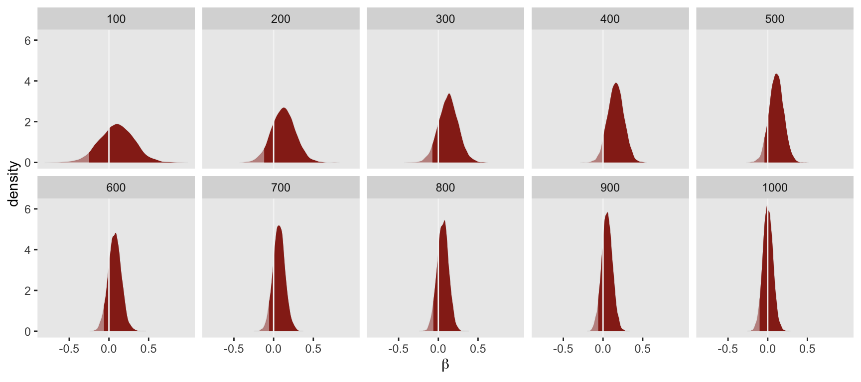
bayes_ci## [1] FALSE FALSE FALSE FALSE FALSE FALSE FALSE FALSE FALSE FALSEHere is a visualization representing the underlying posterior densities at each interim look. It is clear that less than 95% of each density (shaded in darker red) falls to the right of \(0\) at each stage of evaluation, and based on the single decision rule, the study would not have been declared successful at any interim look:

In practice, all we need to do is check whether any of the looks has resulted in a “success”. In this case, there were no successes:
any(bayes_ci)## [1] FALSEOperating characteristics: Type I error rates
Single decision rule
To compare the Type I error rates for each approach, I considered smaller and larger sample sizes:
- 160 subjects, with interim looks every 20 subjects starting after the 80th subject has been enrolled
- 1000 subjects, with interim looks every 100 subjects
For the Bayesian models, I assumed three different prior distribution assumptions for \(\beta\):
\[\beta \sim t_{\text{student}}(\text{df}=3, 0, \sigma), \ \sigma \in \{1, 5, 10\}\]
I generated 3000 data sets under each scenario, and the Type I error rate is the proportion of those 3000 iterations that were declared a “success” under each model. (Code for running these replications on a high performance computing cluster is shown below in the addendum.) Here are the estimates of the error rate using the single criteria for the threshold, comparing the frequentist analysis and the Bayesian analysis.
Type I error rates based on 160 subjects/5 interim looks
##    p_sigma m_effect  freq  bayes
## 1:       1        0 0.118 0.0937
## 2:       5        0 0.099 0.0993
## 3:      10        0 0.101 0.0917
Type I error rates based on 1000 subjects/10 interim looks
##    p_sigma m_effect  freq bayes
## 1:       1        0 0.193 0.157
## 2:       5        0 0.197 0.166
## 3:      10        0 0.189 0.169
At both sample size levels, the Bayesian analysis has a slightly lower Type I error rate compared to the frequentist analysis, although in both cases error rates are considerably inflated beyond 5%. It does not appear that, in this setting at least, that the prior distribution assumptions have much impact on the estimated Type I error rate.
Two crieteria
It is pretty clear in this simple scenario the single Bayesian criterion might not satisfy reviewers looking for control at the 5% level, so we might need to use a modified approach. The next set of simulations explore the double decision rule. In addition to the sample size variation and different prior distribution assumptions, I also considered three possible thresholds for the second criteria in exploring impacts on Type I error rates:
\[P(\beta > 0) > 95\% \ \ \textbf{and} \ \ P(\beta > M) > 50\%, \ M \in \{0.2, 0.3, 0.4\}\]
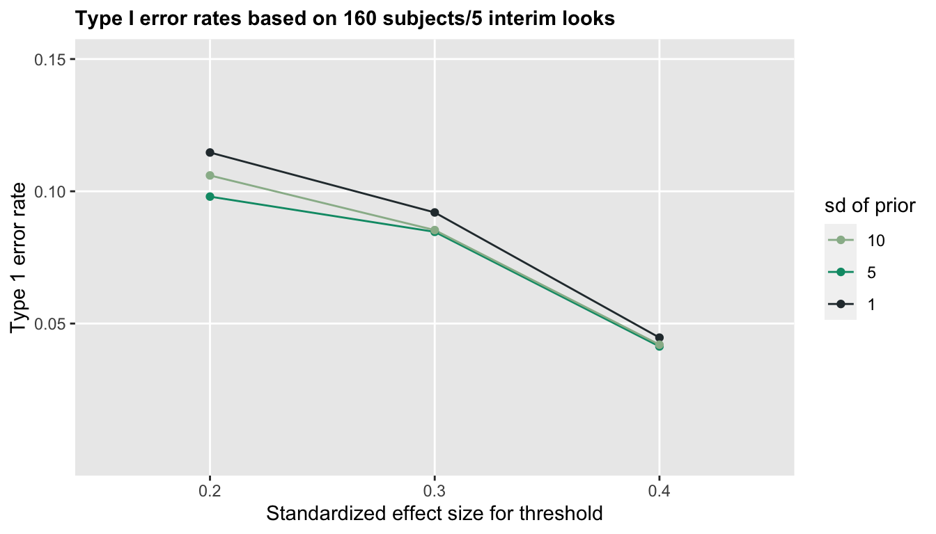
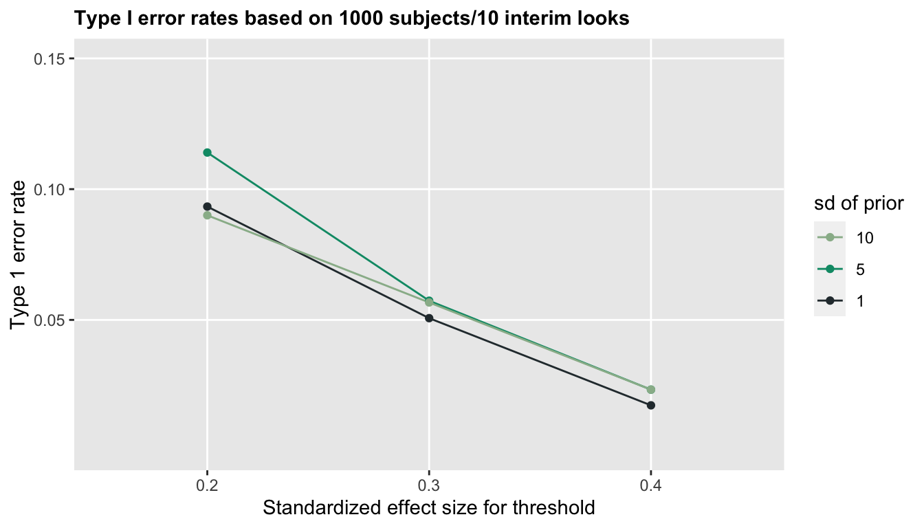
Introducing the second criteria in this case substantially lowers the Type 1 error rate, particularly when the threshold for the second criteria is more conservative (higher):


Once again, the prior distribution assumptions for \(\beta\) are not very important, but the threshold \(M\) is clearly key to controlling the Type I error, particularly when the sample size is smaller. With sample size of 160, 5% error rates are achieved with \(M=0.4\), though with 1000 subjects, we could use \(M=0.3\).
The overall takeaway is that if funders and reviewers insist that Bayesian study designs control Type I error rates at a level of 5%, decision criteria and possibly modelling assumptions might need to be adjusted to accommodate those requirements. This is particularly true if the study design allows for interim evaluations of the data, as is common in a study using an adaptive Bayesian design. Simulations similar to what I have done here will be required to demonstrate that these conditions are satisfied.
References:
Ryan, Elizabeth G., Kristian Brock, Simon Gates, and Daniel Slade. “Do we need to adjust for interim analyses in a Bayesian adaptive trial design?.” BMC medical research methodology 20, no. 1 (2020): 1-9.
Greenland, Sander, Stephen J. Senn, Kenneth J. Rothman, John B. Carlin, Charles Poole, Steven N. Goodman, and Douglas G. Altman. “Statistical tests, P values, confidence intervals, and power: a guide to misinterpretations.” European journal of epidemiology 31, no. 4 (2016): 337-350.
Addendum
Code used to generate p-value estimates for a variety of scenarios was written to be executed on a high performance computing cluster, which is a highly parallel computing environment. I am using package rslurm to manage the parallelization of the process (there is an alternative package called slurmR which I have used in the past). The replications of each of the scenarios (represented by a set of simulation parameters) are stored in data frame scenarios, and the function slurm_apply cycles through the data frame, with many replications executed in parallel. The function s_replication calls the two functions bayes_fit and freq_fit described above.
library(simstudy)
library(data.table)
library(parallel)
library(cmdstanr)
library(posterior)
library(rslurm)

### Function to generate data and estimate parameters

s_replicate <- function(iter, p_sigma, decision_rule, m_effect, seq) {

  set_cmdstan_path(path = "/gpfs/.../cmdstan/2.25.0")

  def <- defData(varname = "rx", formula = "1;1", dist = "trtAssign")
  def <- defData(def, varname = "y", formula = 0, variance = 1, dist = "normal")

  dd <- genData(end, def)

  freq_ps <- sapply(seq(start, end, by = by), function(x) freq_fit(dd[1:x]))
  freq_effect <- any(freq_ps < 0.05)

  bayes_ci <- sapply(seq(start, end, by = by),
    function(x) bayes_fit(dd[1:x], p_sigma, m_effect, decision_rule, x))
  bayes_effect <- any(bayes_ci)

  return(data.table(seq, iter, p_sigma, m_effect, decision_rule,
    freq_effect, bayes_effect))
}

### Set simulation parameters

scenario_dt <- function(...) {
  argdt <- data.table(expand.grid(...))
  argdt[, seq := .I]
  argdt[]
}

iter <- c(1:1000)
p_sigma <- c(1, 5, 10)
decision_rule = 2
m_effect <- c(0.2, 0.3, 0.4) # if decision_rule = 2
# decision_rule = 1
# m_effect <- 0

start <- 100L
end <- 1000L
by <- 100L

scenarios <- scenario_dt(
  iter = iter,
  p_sigma = p_sigma,
  decision_rule = decision_rule,
  m_effect = m_effect
)

### Compile stan code

set_cmdstan_path(path = "/gpfs/.../cmdstan/2.25.0")
mod <- cmdstan_model("multiple.stan")

### Set rslurm arguments

sopts <- list(time = '12:00:00', partition = "cpu_short", `mem-per-cpu` = "5G")
sobjs <- c("freq_fit", "bayes_fit", "mod", "start", "end", "by")

### Replicate over iterations

sjob <- slurm_apply(
  f = s_replicate, # the function
  params = scenarios, # a data frame
  jobname = 'mult_i',
  nodes = 50,
  slurm_options = sopts,
  global_objects = sobjs,
  submit = TRUE
)

### Collect the results and save them

res <- get_slurm_out(sjob, outtype = 'table', wait = TRUE)
save(res, file = "/gpfs/.../mult.rda")