Considering sensitivity to unmeasured confounding: part 2

Two DGPs, same data

Recall from Part 1 that we have an observed data model

\[ Y = k_0 + k_1D + \epsilon_Y\] where \(\epsilon_Y \sim N\left(0, \sigma^2_Y\right)\). We are wondering if there is another DGP that could have generated the data that we have actually observed:

\[ \begin{aligned} D &= \alpha_0 + \alpha_1 U + \epsilon_D \\ Y &= \beta_0 + \beta_1 D + \beta_2 U + \epsilon_{Y^*}, \end{aligned} \]

where \(U\) is some unmeasured confounder, and \(\epsilon_D \sim N\left(0, \sigma^2_D\right)\) and \(\epsilon_{Y^*} \sim N\left(0, \sigma^2_{Y^*}\right)\). Can we go even further and find an alternative DGP where \(D\) has no direct effect on \(Y\) at all?

\[ \begin{aligned} D &= \alpha_0 + \alpha_1 U + \epsilon_D \\ Y &= \beta_0 + \beta_2 U + \epsilon_{Y^*}, \end{aligned} \]

\(\alpha_1\) (and \(\sigma_{\epsilon_D}^2\)) derived from \(\rho_{UD}\)

In a simple linear regression model with a single predictor, the coefficient \(\alpha_1\) can be specified directly in terms \(\rho_{UD}\), the correlation between \(U\) and \(D\):

\[ \alpha_1 = \rho_{UD} \frac{\sigma_D}{\sigma_U}\] We can estimate \(\sigma_D\) from the observed data set, and we can reasonably assume that \(\sigma_U = 1\) (since we could always normalize the original measurement of \(U\)). Finally, we can specify a range of \(\rho_{UD}\) (I am keeping everything positive here for simplicity), such that \(0 < \rho_{UD} < 0.90\) (where I assume a correlation of \(0.90\) is at or beyond the realm of reasonableness). By plugging these three parameters into the formula, we can generate a range of \(\alpha_1\)’s.

Furthermore, we can derive an estimate of the variance for \(\epsilon_D\) ( \(\sigma_{\epsilon_D}^2\)) at each level of \(\rho_{UD}\):

\[ \begin{aligned} Var(D) &= Var(\alpha_0 + \alpha_1 U + \epsilon_D) \\ \\ \sigma_D^2 &= \alpha_1^2 \sigma_U^2 + \sigma_{\epsilon_D}^2 \\ \\ \sigma_{\epsilon_D}^2 &= \sigma_D^2 - \alpha_1^2 \; \text{(since } \sigma_U^2=1) \end{aligned} \]

So, for each value of \(\rho_{UD}\) that we generated, there is a corresponding pair \((\alpha_1, \; \sigma_{\epsilon_D}^2)\).

Determine \(\beta_2\)

In the addendum I go through a bit of an elaborate derivation of \(\beta_2\), the coefficient of \(U\) in the alternative outcome model. Here is the bottom line:

\[ \beta_2 = \frac{\alpha_1}{1-\frac{\sigma_{\epsilon_D}^2}{\sigma_D^2}}\left( k_1 - \beta_1\right) \]

In the equation, we have \(\sigma^2_D\) and \(k_1\), which are both estimated from the observed data and the pair of derived parameters \(\alpha_1\) and \(\sigma_{\epsilon_D}^2\) based on \(\rho_{UD}\). \(\beta_1\), the coefficient of \(D\) in the outcome model is a free parameter, set externally. That is, we can choose to evaluate all \(\beta_2\)’s the are generated when \(\beta_1 = 0\). More generally, we can set \(\beta_1 = pk_1\), where \(0 \le p \le 1\). (We could go negative if we want, though I won’t do that here.) If \(p=1\) , \(\beta_1 = k_1\) and \(\beta_2 = 0\); we end up with the original model with no confounding.

So, once we specify \(\rho_{UD}\) and \(p\), we get the corresponding triplet \((\alpha_1, \; \sigma_{\epsilon_D}^2, \; \beta_2)\).

Determine \(\rho_{UY}\)

In this last step, we can identify the correlation of \(U\) and \(Y\), \(\rho_{UY}\), that is associated with all the observed, specified, and derived parameters up until this point. We start by writing the alternative outcome model, and then replace \(D\) with the alternative exposure model, and do some algebraic manipulation to end up with a re-parameterized alternative outcome model that has a single predictor:

\[ \begin{aligned} Y &= \beta_0 + \beta_1 D + \beta_2 U + \epsilon_Y^* \\ &= \beta_0 + \beta_1 \left( \alpha_0 + \alpha_1 U + \epsilon_D \right) + \beta_2 U + \epsilon_Y^* \\ &=\beta_0 + \beta_1 \alpha_0 + \beta_1 \alpha_1 U + \beta_1 \epsilon_D + \beta_2 U + \epsilon_Y^* \\ &=\beta_0^* + \left( \beta_1 \alpha_1 + \beta_2 \right)U + \epsilon_Y^+ \\ &=\beta_0^* + \beta_1^*U + \epsilon_Y^+ , \\ \end{aligned} \]

where \(\beta_0^* = \beta_0 + \beta_1 \alpha_0\), \(\beta_1^* = \left( \beta_1 \alpha_1 + \beta_2 \right)\), and \(\epsilon_Y^+ = \beta_1 \epsilon_D + \epsilon_Y*\).

As before, the coefficient in a simple linear regression model with a single predictor is related to the correlation of the two variables as follows:

\[ \beta_1^* = \rho_{UY} \frac{\sigma_Y}{\sigma_U} \]

Since \(\beta_1^* = \left( \beta_1 \alpha_1 + \beta_2 \right)\),

\[ \begin{aligned} \beta_1 \alpha_1 + \beta_2 &= \rho_{UY} \frac{\sigma_Y}{\sigma_U} \\ \\ \rho_{UY} &= \frac{\sigma_U}{\sigma_Y} \left( \beta_1 \alpha_1 + \beta_2 \right) \\ \\ &= \frac{\left( \beta_1 \alpha_1 + \beta_2 \right)}{\sigma_Y} \end{aligned} \]

Determine \(\sigma^2_{Y*}\)

In order to simulate data from the alternative DGPs, we need to derive the variation for the noise of the alternative model. That is, we need an estimate of \(\sigma^2_{Y*}\).

\[ \begin{aligned} Var(Y) &= Var(\beta_0 + \beta_1 D + \beta_2 U + \epsilon_{Y^*}) \\ \\ &= \beta_1^2 Var(D) + \beta_2^2 Var(U) + 2\beta_1\beta_2Cov(D, U) + Var(\epsilon_{y*}) \\ \\ &= \beta_1^2 \sigma^2_D + \beta_2^2 + 2\beta_1\beta_2\rho_{UD}\sigma_D + \sigma^2_{Y*} \\ \end{aligned} \]

So,

\[ \sigma^2_{Y*} = Var(Y) - (\beta_1^2 \sigma^2_D + \beta_2^2 + 2\beta_1\beta_2\rho_{UD}\sigma_D), \]

where \(Var(Y)\) is the variation of \(Y\) from the observed data. Now we are ready to implement this in R.

Implementing in R

If we have an observed data set with observed \(D\) and \(Y\), and some target \(\beta_1\) determined by \(p\), we can calculate/generate all the quantities that we just derived.

Before getting to the function, I want to make a brief point about what we do if we have other measured confounders. We can essentially eliminate measured confounders by regressing the exposure \(D\) on the confounders and conducting the entire sensitivity analysis with the residual exposure measurements derived from this initial regression model. I won’t be doing this here, but if anyone wants to see an example of this, let me know, and I can do a short post.

OK - here is the function, which essentially follows the path of the derivation above:

altDGP <- function(dd, p) {
  
  # Create values of rhoUD
  
  dp <- data.table(p = p, rhoUD = seq(0.0, 0.9, length = 1000))
  
  # Parameters estimated from data
  
  dp[, `:=`(sdD = sd(dd$D), s2D = var(dd$D), sdY = sd(dd$Y))] 
  dp[, k1:= coef(lm(Y ~ D, data = dd))[2]]
  
  # Generate b1 based on p
  
  dp[, b1 := p * k1]
  
  # Determine a1
  
  dp[, a1 := rhoUD * sdD ]
  
  # Determine s2ed
  
  dp[, s2ed := s2D - (a1^2)]
  
  # Determine b2
  
  dp[, g:= s2ed/s2D]
  dp <- dp[g != 1]
  dp[, b2 := (a1 / (1 - g) ) * ( k1 - b1 )]
  
  # Determine rhoUY
  
  dp[, rhoUY := ( (b1 * a1) + b2 ) / sdY ]
  
  # Eliminate impossible correlations
  
  dp <- dp[rhoUY > 0 & rhoUY <= .9]
  
  # Determine s2eyx
  
  dp[, s2eyx := sdY^2 - (b1^2 * s2D + b2^2 + 2 * b1 * b2 * rhoUD * sdD)]
  dp <- dp[s2eyx > 0]
  
  # Determine standard deviations
  
  dp[, sdeyx := sqrt(s2eyx)]
  dp[, sdedx := sqrt(s2ed)]
  
  # Finished
  
  dp[]
  
}

Assessing sensitivity

If we generate the same data set we started out with last post, we can use the function to assess the sensitivity of this association.

defO <- defData(varname = "D", formula = 0, variance = 1)
defO <- defData(defO, varname = "Y", formula = "1.5 * D", variance = 25)

set.seed(20181201)
dtO <- genData(1200, defO)

In this first example, I am looking for the DGP with \(\beta_1 = 0\), which is implemented as \(p = 0\) in the call to function altDGP. Each row of output represents an alternative set of parameters that will result in a DGP with \(\beta_1 = 0\).

dp <- altDGP(dtO, p = 0)
dp[, .(rhoUD, rhoUY, k1, b1, a1, s2ed, b2, s2eyx)]

##      rhoUD rhoUY   k1 b1    a1  s2ed   b2 s2eyx
##   1: 0.295 0.898 1.41  0 0.294 0.904 4.74  5.36
##   2: 0.296 0.896 1.41  0 0.295 0.903 4.72  5.50
##   3: 0.297 0.893 1.41  0 0.296 0.903 4.71  5.63
##   4: 0.298 0.890 1.41  0 0.297 0.902 4.69  5.76
##   5: 0.299 0.888 1.41  0 0.298 0.902 4.68  5.90
##  ---                                           
## 668: 0.896 0.296 1.41  0 0.892 0.195 1.56 25.35
## 669: 0.897 0.296 1.41  0 0.893 0.193 1.56 25.35
## 670: 0.898 0.296 1.41  0 0.894 0.191 1.56 25.36
## 671: 0.899 0.295 1.41  0 0.895 0.190 1.56 25.36
## 672: 0.900 0.295 1.41  0 0.896 0.188 1.55 25.37

Now, I am creating a data set that will be based on four levels of \(\beta_1\). I do this by creating a vector \(p = \; <0.0, \; 0.2, \; 0.5, \; 0.8>\). The idea is to create a plot that shows the curve for each value of \(p\). The most extreme curve (in this case, the curve all the way to the right, since we are dealing with positive associations only) represents the scenario where \(p = 0\) (i.e. \(\beta_1 = 0\)). The curves moving to the left reflect increasing sensitivity as \(p\) increases.

dsenO <- rbindlist(lapply(c(0.0, 0.2, 0.5, 0.8), 
                     function(x) altDGP(dtO, x)))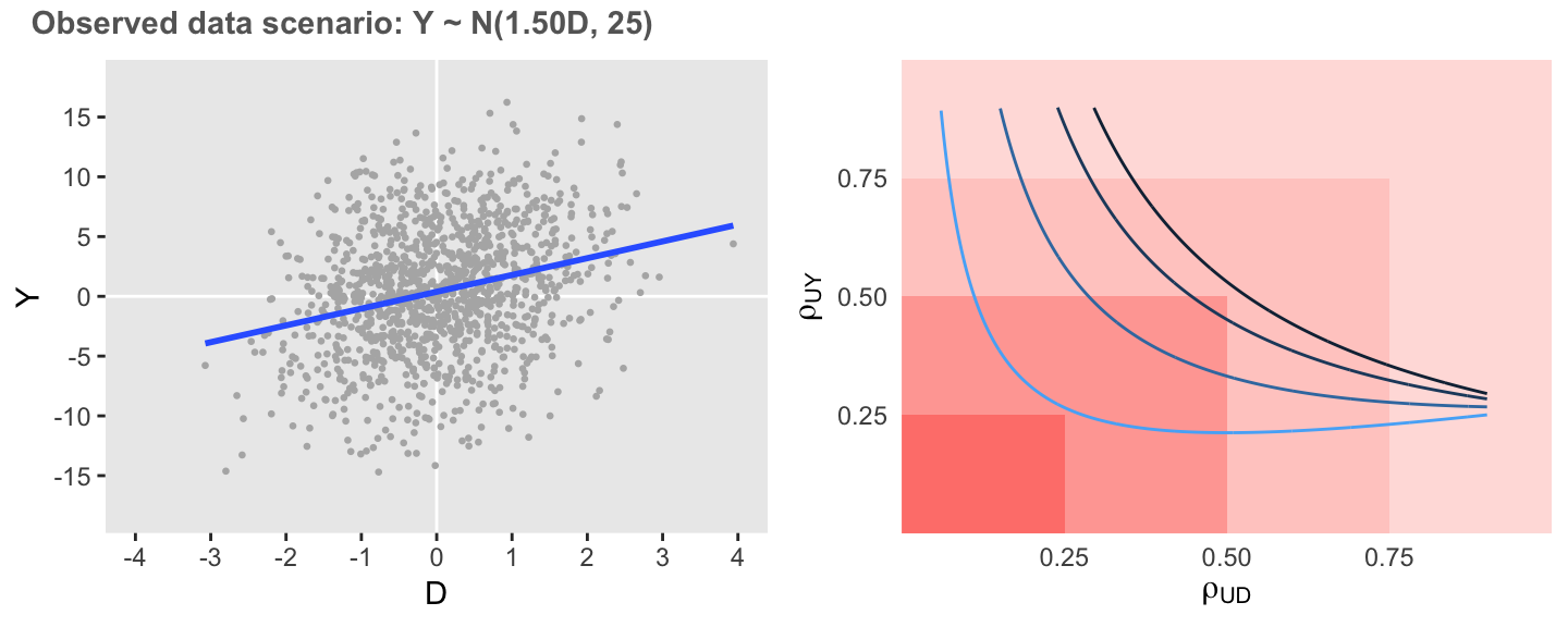

I would say that in this first case the observed association is moderately sensitive to unmeasured confounding, as correlations as low as 0.5 would enough to erase the association.

In the next case, if the association remains unchanged but the variation of \(Y\) is considerably reduced, the observed association is much less sensitive. However, it is still quite possible that the observed overestimation is at least partially overstated, as relatively low levels of correlation could reduce the estimated association.

defA1 <- updateDef(defO, changevar = "Y", newvariance = 4)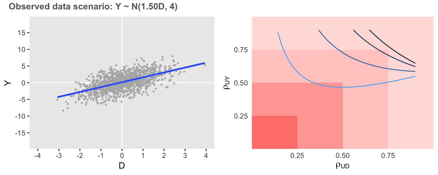

In this last scenario, variance is the same as the initial scenario, but the association is considerably weaker. Here, we see that the estimate of the association is extremely sensitive to unmeasured confounding, as low levels of correlation are required to entirely erase the association.

defA2 <- updateDef(defO, changevar = "Y", newformula = "0.25 * D")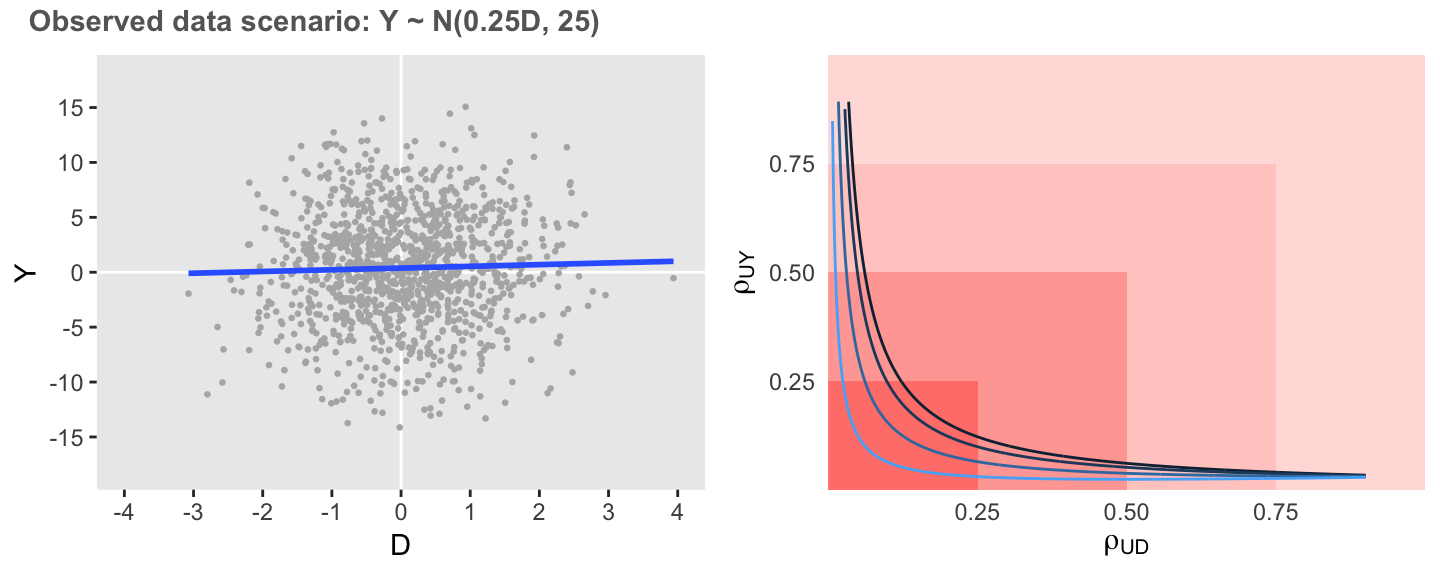

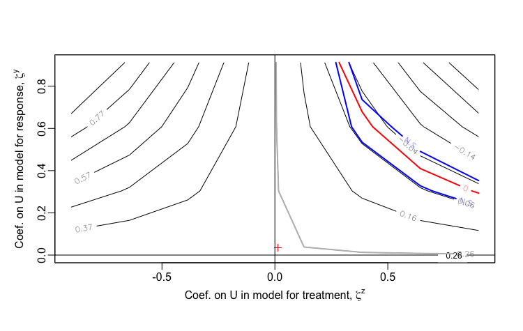
treatSens package

I want to show output generated by the treatSens package I referenced earlier. treatSens requires a formula that includes an outcome vector \(Y\), an exposure vector \(Z\), and at least one vector of measured of confounders \(X\). In my examples, I have included no measured confounders, so I generate a vector of independent noise that is not related to the outcome.

library(treatSens)

X <- rnorm(1200)
Y <- dtO$Y
Z <- dtO$D

testsens <- treatSens(Y ~ Z + X, nsim = 5)
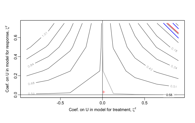
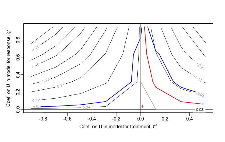
sensPlot(testsens)

Once treatSens has been executed, it is possible to generate a sensitivity plot, which looks substantively similar to the ones I have created. The package uses sensitivity parameters \(\zeta^Z\) and \(\zeta^Y\), which represent the coefficients of \(U\), the unmeasured confounder. Since treatSens normalizes the data (in the default setting), these coefficients are actually equivalent to the correlations \(\rho_{UD}\) and \(\rho_{UY}\) that are the basis of my sensitivity analysis. A important difference in the output is that treatSens provides uncertainty bands, and extends into regions of negative correlation. (And of course, a more significant difference is that treatSens is flexible enough to handle binary exposures, whereas I have not yet extended my analytic approach in that direction, and I suspect it is no possible for me to do so due to non-collapsibility of logistic regression estimands - I hope to revisit this in the future.)

Addendum: Derivation of \(\beta_2\)

In case you want more detail on how we derive \(\beta_2\) from the observed data model and assumed correlation parameters, here it is. We start by specifying the simple observed outcome model:

\[ Y = k_0 + k_1D + \epsilon_Y\]

We can estimate the parameters \(k_0\) and \(k_1\) using this standard matrix solution:

\[ <k_0, \; k_1> \; = (W^TW)^{-1}W^TY,\]

where \(W\) is the \(n \times 2\) design matrix:

\[ W = [\mathbf{1}, D]_{n \times 2}.\]

We can replace \(Y\) with the alternative outcome model:

\[ \begin{aligned} <k_0, \; k_1> \; &= (W^TW)^{-1}W^T(\beta_0 + \beta_1 D + \beta_2 U + \epsilon_Y^*) \\ &= \;<\beta_0, 0> + <0, \beta_1> +\; (W^TW)^{-1}W^T(\beta_2U) + \mathbf{0} \\ &= \;<\beta_0, \beta_1> +\; (W^TW)^{-1}W^T(\beta_2U) \end{aligned} \]

Note that

\[ \begin{aligned} (W^TW)^{-1}W^T(\beta_0) &= \; <\beta_0,\; 0> \; \; and\\ \\ (W^TW)^{-1}W^T(\beta_1D) &= \; <0,\; \beta_1>. \end{aligned} \]

Now, we need to figure out what \((W^TW)^{-1}W^T(\beta_2U)\) is. First, we rearrange the alternate exposure model: \[ \begin{aligned} D &= \alpha_0 + \alpha_1 U + \epsilon_D \\ \alpha_1 U &= D - \alpha_0 - \epsilon_D \\ U &= \frac{1}{\alpha_1} \left( D - \alpha_0 - \epsilon_D \right) \\ \beta_2 U &= \frac{\beta_2}{\alpha_1} \left( D - \alpha_0 - \epsilon_D \right) \end{aligned} \]

We can replace \(\beta_2 U\):

\[ \begin{aligned} (W^TW)^{-1}W^T(\beta_2U) &= (W^TW)^{-1}W^T \left[ \frac{\beta_2}{\alpha_1} \left( D - \alpha_0 - \epsilon_D \right) \right] \\ &= <-\frac{\beta_2}{\alpha_1}\alpha_0, 0> + <0,\frac{\beta_2}{\alpha_1}>-\;\frac{\beta_2}{\alpha_1}(W^TW)^{-1}W^T \epsilon_D \\ &= <-\frac{\beta_2}{\alpha_1}\alpha_0, \frac{\beta_2}{\alpha_1}>-\;\frac{\beta_2}{\alpha_1}(W^TW)^{-1}W^T \epsilon_D \\ \end{aligned} \]

And now we get back to \(<k_0,\; k_1>\) :

\[ \begin{aligned} <k_0,\; k_1> \; &= \;<\beta_0,\; \beta_1> +\; (W^TW)^{-1}W^T(\beta_2U) \\ &= \;<\beta_0-\frac{\beta_2}{\alpha_1}\alpha_0, \; \beta_1 + \frac{\beta_2}{\alpha_1}>-\;\frac{\beta_2}{\alpha_1}(W^TW)^{-1}W^T \epsilon_D \\ &= \;<\beta_0-\frac{\beta_2}{\alpha_1}\alpha_0, \; \beta_1 + \frac{\beta_2}{\alpha_1}>-\;\frac{\beta_2}{\alpha_1}<\gamma_0, \; \gamma_1> \end{aligned} \]

where \(\gamma_0\) and \(\gamma_1\) come from regressing \(\epsilon_D\) on \(D\):

\[ \epsilon_D = \gamma_0 + \gamma_1 D\] so,

\[ \begin{aligned} <k_0,\; k_1> \; &= \;<\beta_0-\frac{\beta_2}{\alpha_1}\alpha_0 - \frac{\beta_2}{\alpha_1}\gamma_0, \; \beta_1 + \frac{\beta_2}{\alpha_1} - \frac{\beta_2}{\alpha_1}\gamma_1 > \\ &= \;<\beta_0-\frac{\beta_2}{\alpha_1}\left(\alpha_0 + \gamma_0\right), \; \beta_1 + \frac{\beta_2}{\alpha_1}\left(1 - \gamma_1 \right) > \end{aligned} \]

Since we can center all the observed data, we can easily assume that \(k_0 = 0\). All we need to worry about is \(k_1\):

\[ \begin{aligned} k_1 &= \beta_1 + \frac{\beta_2}{\alpha_1}\left(1 - \gamma_1 \right) \\ \frac{\beta_2}{\alpha_1}\left(1 - \gamma_1 \right) &= k_1 - \beta_1 \\ \beta_2 &= \frac{\alpha_1}{1-\gamma_1}\left( k_1 - \beta_1\right) \end{aligned} \]

We have generated \(\alpha_1\) based on \(\rho_{UD}\), \(k_1\) is a estimated from the data, and \(\beta_1\) is fixed based on some \(p, \; 0 \le p \le 1\) such that \(\beta_1 = pk_1\). All that remains is \(\gamma_1\):

\[ \gamma_1 = \rho_{\epsilon_D D} \frac{\sigma_{\epsilon_D}}{\sigma_D} \]

Since \(D = \alpha_0 + \alpha_1 U + \epsilon_D\) (and \(\epsilon_D \perp \! \! \! \perp U\))

\[ \begin{aligned} \rho_{\epsilon_D D} &= \frac{Cov(\epsilon_D, D)}{\sigma_{\epsilon_D} \sigma_D} \\ \\ &=\frac{Cov(\epsilon_D, \;\alpha_0 + \alpha_1 U + \epsilon_D )}{\sigma_{\epsilon_D} \sigma_D} \\ \\ &= \frac{\sigma_{\epsilon_D}^2}{\sigma_{\epsilon_D} \sigma_D} \\ \\ &= \frac{\sigma_{\epsilon_D}}{\sigma_D} \end{aligned} \]

It follows that

\[ \begin{aligned} \gamma_1 &= \rho_{\epsilon_D D} \frac{\sigma_{\epsilon_D}}{\sigma_D} \\ \\ &=\frac{\sigma_{\epsilon_D}}{\sigma_D} \times \frac{\sigma_{\epsilon_D}}{\sigma_D} \\ \\ &=\frac{\sigma_{\epsilon_D}^2}{\sigma_D^2} \end{aligned} \]

So, now, we have all the elements to generate \(\beta_2\) for a range of \(\alpha_1\)’s and \(\sigma_{\epsilon_D}^2\)’s:

\[ \beta_2 = \frac{\alpha_1}{1-\frac{\sigma_{\epsilon_D}^2}{\sigma_D^2}}\left( k_1 - \beta_1\right) \]