An updated version of the simstudy package (0.1.10) is now available on CRAN. The impetus for this release was a series of requests about generating correlated binary outcomes. In the last post, I described a beta-binomial data generating process that uses the recently added beta distribution. In addition to that update, I’ve added functionality to genCorGen and addCorGen, functions which generate correlated data from non-Gaussian or normally distributed data such as Poisson, Gamma, and binary data. Most significantly, there is a newly implemented algorithm based on the work of Emrich & Piedmonte, which I mentioned the last time around.
Limitation of copula algorithm
The existing copula algorithm is limited when generating correlated binary data. (I did acknowledge this when I first introduced the new functions.) The generated marginal means are what we would expect. though the observed correlation on the binary scale is biased downwards towards zero. Using the copula algorithm, the specified correlation really pertains to the underlying normal data that is used in the data generation process. Information is lost when moving between the continuous and dichotomous distributions:
library(simstudy)

set.seed(736258)
d1 <- genCorGen(n = 1000, nvars = 4, params1 = c(0.2, 0.5, 0.6, 0.7),
                dist = "binary", rho = 0.3, corstr = "cs", wide = TRUE,
                method = "copula")

d1
## id V1 V2 V3 V4
## 1: 1 0 0 0 0
## 2: 2 0 1 1 1
## 3: 3 0 1 0 1
## 4: 4 0 0 1 0
## 5: 5 0 1 0 1
## ---
## 996: 996 0 0 0 0
## 997: 997 0 1 0 0
## 998: 998 0 1 1 1
## 999: 999 0 0 0 0
## 1000: 1000 0 0 0 0d1[, .(V1 = mean(V1), V2 = mean(V2),
V3 = mean(V3), V4 = mean(V4))]## V1 V2 V3 V4
## 1: 0.184 0.486 0.595 0.704d1[, round(cor(cbind(V1, V2, V3, V4)), 2)]## V1 V2 V3 V4
## V1 1.00 0.18 0.17 0.17
## V2 0.18 1.00 0.19 0.23
## V3 0.17 0.19 1.00 0.15
## V4 0.17 0.23 0.15 1.00The ep option offers an improvement
Data generated using the Emrich & Piedmonte algorithm, done by specifying the “ep” method, does much better; the observed correlation is much closer to what we specified. (Note that the E&P algorithm may restrict the range of possible correlations; if you specify a correlation outside of the range, an error message is issued.)
set.seed(736258)
d2 <- genCorGen(n = 1000, nvars = 4, params1 = c(0.2, 0.5, 0.6, 0.7),
                dist = "binary", rho = 0.3, corstr = "cs", wide = TRUE,
                method = "ep")

d2[, .(V1 = mean(V1), V2 = mean(V2),
       V3 = mean(V3), V4 = mean(V4))]
## V1 V2 V3 V4
## 1: 0.199 0.504 0.611 0.706d2[, round(cor(cbind(V1, V2, V3, V4)), 2)]## V1 V2 V3 V4
## V1 1.00 0.33 0.33 0.29
## V2 0.33 1.00 0.32 0.31
## V3 0.33 0.32 1.00 0.28
## V4 0.29 0.31 0.28 1.00If we generate the data using the “long” form, we can fit a GEE marginal model to recover the parameters used in the data generation process:
library(geepack)

set.seed(736258)
d3 <- genCorGen(n = 1000, nvars = 4, params1 = c(0.2, 0.5, 0.6, 0.7),
                dist = "binary", rho = 0.3, corstr = "cs", wide = FALSE,
                method = "ep")

geefit3 <- geeglm(X ~ factor(period), id = id, data = d3,
                  family = binomial, corstr = "exchangeable")

summary(geefit3)
##
## Call:
## geeglm(formula = X ~ factor(period), family = binomial, data = d3,
## id = id, corstr = "exchangeable")
##
## Coefficients:
## Estimate Std.err Wald Pr(>|W|)
## (Intercept) -1.39256 0.07921 309.1 <2e-16 ***
## factor(period)1 1.40856 0.08352 284.4 <2e-16 ***
## factor(period)2 1.84407 0.08415 480.3 <2e-16 ***
## factor(period)3 2.26859 0.08864 655.0 <2e-16 ***
## ---
## Signif. codes: 0 '***' 0.001 '**' 0.01 '*' 0.05 '.' 0.1 ' ' 1
##
## Estimated Scale Parameters:
## Estimate Std.err
## (Intercept) 1 0.01708
##
## Correlation: Structure = exchangeable Link = identity
##
## Estimated Correlation Parameters:
## Estimate Std.err
## alpha 0.3114 0.01855
## Number of clusters: 1000 Maximum cluster size: 4And the point estimates for each variable on the probability scale:
round(1/(1+exp(1.3926 - c(0, 1.4086, 1.8441, 2.2686))), 2)## [1] 0.20 0.50 0.61 0.71Longitudinal (repeated) measures
One researcher wanted to generate individual-level longitudinal data that might be analyzed using a GEE model. This is not so different from what I just did, but incorporates a specific time trend to define the probabilities. In this case, the steps are to (1) generate longitudinal data using the addPeriods function, (2) define the longitudinal probabilities, and (3) generate correlated binary outcomes with an AR-1 correlation structure.
set.seed(393821)
probform <- "-2 + 0.3 * period"

def1 <- defDataAdd(varname = "p", formula = probform,
                   dist = "nonrandom", link = "logit")

dx <- genData(1000)
dx <- addPeriods(dx, nPeriods = 4)
dx <- addColumns(def1, dx)

dg <- addCorGen(dx, nvars = 4,
                corMatrix = NULL, rho = .4, corstr = "ar1",
                dist = "binary", param1 = "p",
                method = "ep", formSpec = probform,
                periodvar = "period")
The correlation matrix from the observed data is reasonably close to having an AR-1 structure, where \(\rho = 0.4\), \(\rho^2 = 0.16\), \(\rho^3 = 0.064\).
cor(dcast(dg, id ~ period, value.var = "X")[,-1])## 0 1 2 3
## 0 1.00000 0.4309 0.1762 0.04057
## 1 0.43091 1.0000 0.3953 0.14089
## 2 0.17618 0.3953 1.0000 0.36900
## 3 0.04057 0.1409 0.3690 1.00000And again, the model recovers the time trend parameter defined in variable probform as well as the correlation parameter:
geefit <- geeglm(X ~ period, id = id, data = dg, corstr = "ar1",
                 family = binomial)
summary(geefit)
##
## Call:
## geeglm(formula = X ~ period, family = binomial, data = dg, id = id,
## corstr = "ar1")
##
## Coefficients:
## Estimate Std.err Wald Pr(>|W|)
## (Intercept) -1.9598 0.0891 484.0 <2e-16 ***
## period 0.3218 0.0383 70.6 <2e-16 ***
## ---
## Signif. codes: 0 '***' 0.001 '**' 0.01 '*' 0.05 '.' 0.1 ' ' 1
##
## Estimated Scale Parameters:
## Estimate Std.err
## (Intercept) 1 0.0621
##
## Correlation: Structure = ar1 Link = identity
##
## Estimated Correlation Parameters:
## Estimate Std.err
## alpha 0.397 0.0354
## Number of clusters: 1000 Maximum cluster size: 4Model mis-specification
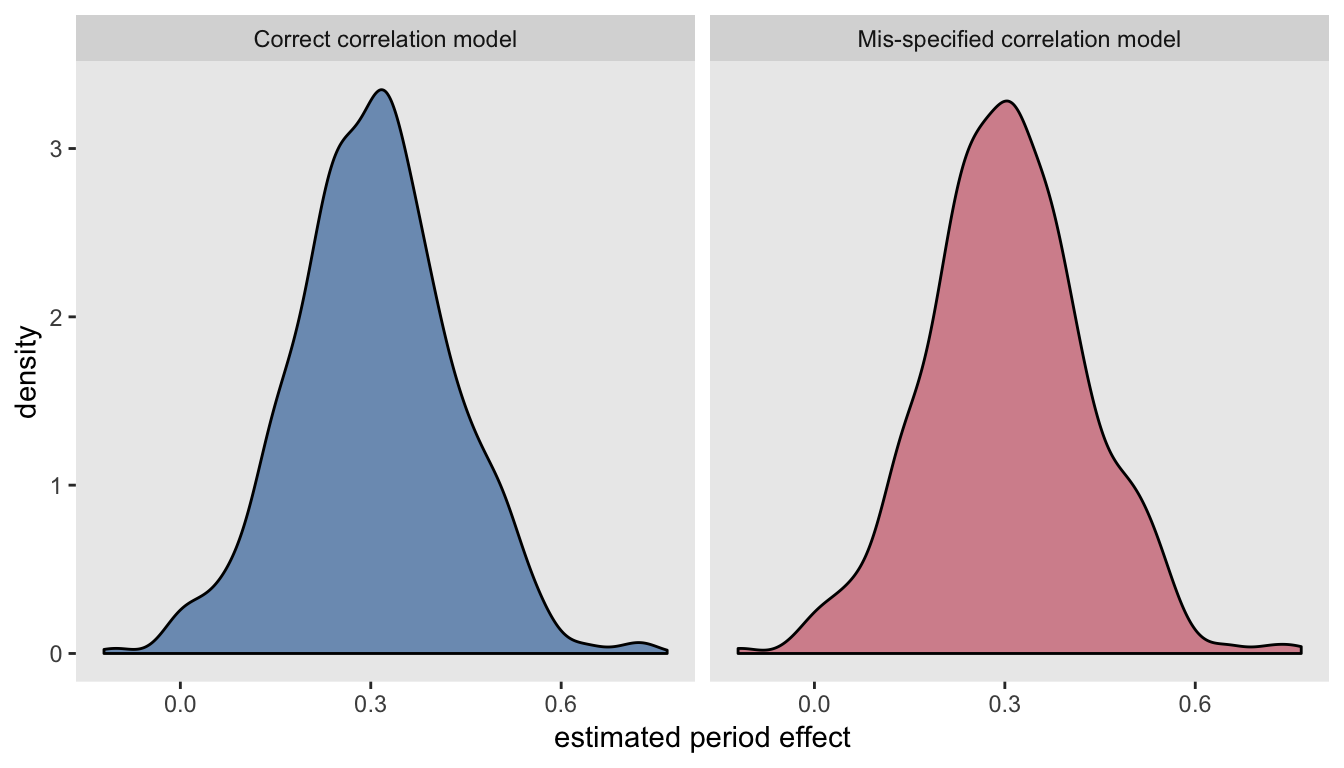
And just for fun, here is an example of how simulation might be used to investigate the performance of a model. Let’s say we are interested in the implications of mis-specifying the correlation structure. In this case, we can fit two GEE models (one correctly specified and one mis-specified) and assess the sampling properties of the estimates from each:
library(broom)

dx <- genData(100)
dx <- addPeriods(dx, nPeriods = 4)
dx <- addColumns(def1, dx)

iter <- 1000
rescorrect <- vector("list", iter)
resmisspec <- vector("list", iter)

for (i in 1:iter) {

  dw <- addCorGen(dx, nvars = 4,
                  corMatrix = NULL, rho = .5, corstr = "ar1",
                  dist = "binary", param1 = "p",
                  method = "ep", formSpec = probform,
                  periodvar = "period")

  correctfit <- geeglm(X ~ period, id = id, data = dw,
                       corstr = "ar1", family = binomial)

  misfit     <- geeglm(X ~ period, id = id, data = dw,
                       corstr = "independence", family = binomial)

  rescorrect[[i]] <- data.table(i, tidy(correctfit))
  resmisspec[[i]] <- data.table(i, tidy(misfit))
}

rescorrect <-
  rbindlist(rescorrect)[term == "period"][, model := "correct"]

resmisspec <-
  rbindlist(resmisspec)[term == "period"][, model := "misspec"]
Here are the averages, standard deviation, and average standard error of the point estimates under the correct specification:
rescorrect[, c(mean(estimate), sd(estimate), mean(std.error))]## [1] 0.304 0.125 0.119And for the incorrect specification:
resmisspec[, c(mean(estimate), sd(estimate), mean(std.error))]## [1] 0.303 0.126 0.121The estimates of the time trend from both models are unbiased, and the observed standard error of the estimates are the same for each model, which in turn are not too far off from the estimated standard errors. This becomes quite clear when we look at the virtually identical densities of the estimates:
Addendum
As an added bonus, here is a conditional generalized mixed effects model of the larger data set generated earlier. The conditional estimates are quite different from the marginal GEE estimates, but this is not surprising given the binary outcomes. (For comparison, the period coefficient was estimated using the marginal model to be 0.32)
library(lme4)

glmerfit <- glmer(X ~ period + (1 | id), data = dg, family = binomial)
summary(glmerfit)
## Generalized linear mixed model fit by maximum likelihood (Laplace
## Approximation) [glmerMod]
## Family: binomial ( logit )
## Formula: X ~ period + (1 | id)
## Data: dg
##
## AIC BIC logLik deviance df.resid
## 3595 3614 -1795 3589 3997
##
## Scaled residuals:
## Min 1Q Median 3Q Max
## -1.437 -0.351 -0.284 -0.185 2.945
##
## Random effects:
## Groups Name Variance Std.Dev.
## id (Intercept) 2.38 1.54
## Number of obs: 4000, groups: id, 1000
##
## Fixed effects:
## Estimate Std. Error z value Pr(>|z|)
## (Intercept) -2.7338 0.1259 -21.7 <2e-16 ***
## period 0.4257 0.0439 9.7 <2e-16 ***
## ---
## Signif. codes: 0 '***' 0.001 '**' 0.01 '*' 0.05 '.' 0.1 ' ' 1
##
## Correlation of Fixed Effects:
## (Intr)
## period -0.700