simstudy just got a little more dynamic: version 0.2.1

Double-dot external variable reference

It may be useful to think of an external reference variable as a type of hyperparameter of the data generation process. The reference is made directly in the formula itself, using a double-dot (“..”) notation before the variable name.

Here is a simple example:

library(simstudy)

def <- defData(varname = "x", formula = 0, 
  variance = 5, dist = "normal")
def <- defData(def, varname = "y", formula = "..B0 + ..B1 * x", 
  variance = "..sigma2", dist = "normal")

def

##    varname         formula variance   dist     link
## 1:       x               0        5 normal identity
## 2:       y ..B0 + ..B1 * x ..sigma2 normal identity

B0, B1, and sigma2 are not part of the simstudy data definition, but will be set external to that process, either in the global environment or within the context of a function.

B0 <- 4;
B1 <- 2;
sigma2 <- 9

set.seed(716251)
dd <- genData(100, def)

fit <- summary(lm(y ~ x, data = dd))

coef(fit)

##             Estimate Std. Error t value Pr(>|t|)
## (Intercept)        4       0.28      14  2.6e-25
## x                  2       0.13      15  5.9e-28

fit$sigma

## [1] 2.8

It is easy to create a new data set on the fly with different slope and variance assumptions without having to go to the trouble of updating the data definitions.

B1 <- 3
sigma2 <- 16

dd <- genData(100, def)
fit <- summary(lm(y ~ x, data = dd))

coef(fit)

##             Estimate Std. Error t value Pr(>|t|)
## (Intercept)      4.4       0.43      10  4.6e-17
## x                3.1       0.22      14  8.6e-26

fit$sigma

## [1] 4.2

Using with apply functions

Double-dot references can be flexibly applied using lapply (or the parallel version mclapply) to create a range of data sets under different assumptions:

gen_data <- function(sigma2, d) {
  dd <- genData(400, d)
  dd[, sigma2 := sigma2]
  dd
}

sigma2s <- c(1:9)^2

dd_m <- lapply(sigma2s, function(s) gen_data(s, def))
dd_m <- rbindlist(dd_m)

ggplot(data = dd_m, aes(x = x, y = y)) +
  geom_point(size = .5, color = "#DDAA33") +
  facet_wrap(sigma2 ~ .) +
  theme(panel.grid = element_blank())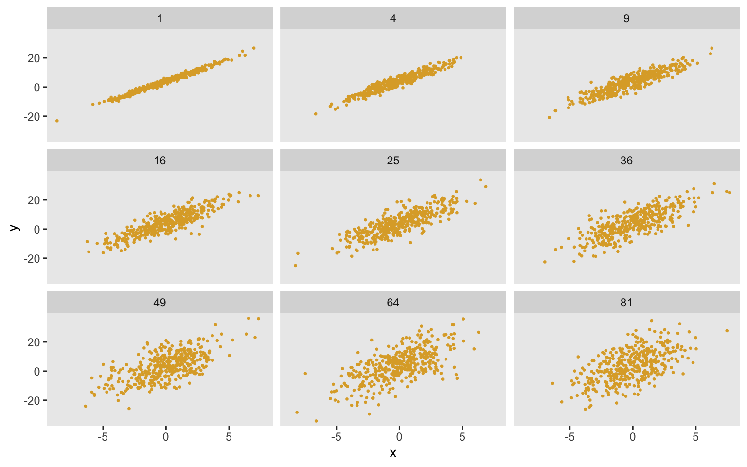

Using with vectors

Double-dot referencing is also vector friendly. For example, if we want to create a mixture distribution from a vector of values (which we can also do using a categorical distribution), we can define the mixture formula in terms of the vector. In this case we are generating permuted block sizes of 2 and 4:

defblk <- defData(varname = "blksize", 
   formula = "..sizes[1] | .5 + ..sizes[2] | .5", dist = "mixture")

defblk

##    varname                           formula variance    dist     link
## 1: blksize ..sizes[1] | .5 + ..sizes[2] | .5        0 mixture identity

sizes <- c(2, 4)
genData(1000, defblk)

##         id blksize
##    1:    1       2
##    2:    2       4
##    3:    3       2
##    4:    4       4
##    5:    5       4
##   ---             
##  996:  996       4
##  997:  997       2
##  998:  998       4
##  999:  999       4
## 1000: 1000       4

There are a few other changes to the package that are described here (but look for version 0.2.0 - we found a pretty major bug right away and fixed it, hence 0.2.1). Moving forward, we have some more things in the works, of course. And if you have suggestions of your own, you know where to find us.

Addendum

Here’s a more detailed example to show how double-dot references simplify things considerably in a case where I originally used the updateDef function. In a post where I described regression to the mean, there is an addendum that I adapt here using double-dot references. I’m not going into the motivation for the code here - check out the post if you’d like to see more.)

Here’s the data original code (both examples require the parallel package):

d <- defData(varname = "U", formula = "-1;1", dist = "uniform")
d <- defData(d, varname = "x1", formula = "0 + 2*U", variance = 1)
d <- defData(d, varname = "x2", formula = "0 + 2*U", variance = 1)
d <- defData(d, varname = "h1", formula = "x1 > quantile(x1, .80) ", 
             dist = "nonrandom")

rtomean <- function(n, d) {
  dd <- genData(n, d)
  data.table(x1 = dd[x1 >= h1, mean(x1)] , x2 = dd[x1 >= h1, mean(x2)])
}

repl <- function(xvar, nrep, ucoef, d) {
  
  d <- updateDef(d, "x1", newvariance = xvar)
  d <- updateDef(d, "x2", newvariance = xvar)
  
  dif <- rbindlist(mclapply(1:nrep, function(x) rtomean(200, d)))
  mudif <- unlist(lapply(dif, mean))
  data.table(ucoef, xvar, x1 = mudif[1], x2 = mudif[2])
  
}

dres <- list()
i <- 0

for (ucoef in c(0, 1, 2, 3)) {
  
  i <- i + 1
  
  uform <- genFormula( c(0, ucoef), "U")
  
  d <- updateDef(d, "x1", newformula = uform)
  d <- updateDef(d, "x2", newformula = uform)
  
  dr <- mclapply(seq(1, 4, by = 1), function(x) repl(x, 1000, ucoef, d))
  dres[[i]] <- rbindlist(dr)
}

dres <- rbindlist(dres)

And here is the updated code:

d <- defData(varname = "U", formula = "-1;1", dist = "uniform")
d <- defData(d, varname = "x1", formula = "0 + ..ucoef*U", variance = "..xvar")
d <- defData(d, varname = "x2", formula = "0 + ..ucoef*U", variance = "..xvar")
d <- defData(d, varname = "h1", formula = "x1 > quantile(x1, .80) ", 
             dist = "nonrandom")

rtomean <- function(n, d, ucoef, xvar) {
  
  dd <- genData(n, d)
  data.table(x1 = dd[x1 >= h1, mean(x1)] , x2 = dd[x1 >= h1, mean(x2)])
  
}

repl <- function(nrep, d, ucoef, xvar) {
  
  dif <- rbindlist(mclapply(1:nrep, function(x) rtomean(200, d, ucoef, xvar)))
  mudif <- unlist(lapply(dif, mean))
  data.table(ucoef, xvar, x1 = mudif[1], x2 = mudif[2])
  
}

ucoef <- c(0:3)
xvar <- c(1:4)
params <- asplit(expand.grid(ucoef = ucoef, xvar = xvar), 1)

dres <- rbindlist(mclapply(params, function(x) repl(1000, d, x["ucoef"], x["xvar"])))

The code is much cleaner and the data generating process doesn’t really lose any clarity. Importantly, this change has allowed me to take advantage of the apply approach (rather than using a loop). I’d conclude that double-dot references have the potential to simplify things quite a bit.