Simulating a cost-effectiveness analysis to highlight new functions for generating correlated data

Simulation scenario

In the simulation scenario I’ve concocted, the goal is to increase the number of patients that come in for an important test. A group of public health professionals have developed a new outreach program that they think will be able to draw in more patients. The study is conducted at the site level - some sites will implement the new approach, and the others, serving as controls, will continue with the existing approach. The cost for the new approach is expected to be higher, and will vary by site. In the first scenario, we assume that costs and recruitment are correlated with each other. That is, sites that tend to spend more generally have higher recruitment levels, even before introducing the new recruitment method.

The data are simulated using the assumption that costs have a gamma distribution (since costs are positive, continuous and skewed to the right) and that recruitment numbers are Poisson distributed (since they are non-negative counts). The intervention sites will have costs that are on average $1000 greater than the control sites. Recruitment will be 10 patients higher for the intervention sites. This is an average expenditure of $100 per additional patient recruited:

library(simstudy)

# Total of 500 sites, 250 control/250 intervention

set.seed(2018)
dt <- genData(500)
dt <- trtAssign(dtName = dt, nTrt = 2, 
                balanced = TRUE, grpName = "trtSite")

# Define data - intervention costs $1000 higher on average

def <- defDataAdd(varname = "cost", formula = "1000 + 1000*trtSite", 
                  variance = 0.2, dist = "gamma")

def <- defDataAdd(def, varname = "nRecruits", 
                  formula = "100 + 10*trtSite", 
                  dist = "poisson")

# Set correlation paramater (based on Kendall's tau)

tau <- 0.2

# Generate correlated data using new function addCorFlex

dOutcomes <- addCorFlex(dt, defs = def, tau = tau)
dOutcomes

##       id trtSite      cost nRecruits
##   1:   1       1 1553.7862        99
##   2:   2       1  913.2466        90
##   3:   3       1 1314.5522        91
##   4:   4       1 1610.5535       112
##   5:   5       1 3254.1100        99
##  ---                                
## 496: 496       1 1452.5903        99
## 497: 497       1  292.8769       109
## 498: 498       0  835.3930        85
## 499: 499       1 1618.0447        92
## 500: 500       0  363.2429       101

The data have been generated, so now we can examine the means and standard deviations of costs and recruitment:

dOutcomes[, .(meanCost = mean(cost), sdCost = sd(cost)), 
          keyby = trtSite]

##    trtSite  meanCost   sdCost
## 1:       0  992.2823 449.8359
## 2:       1 1969.2057 877.1947

dOutcomes[, .(meanRecruit = mean(nRecruits), sdRecruit = sd(nRecruits)), 
          keyby = trtSite]

##    trtSite meanRecruit sdRecruit
## 1:       0      99.708  10.23100
## 2:       1     108.600  10.10308

And here is the estimate of Kendall’s tau within each intervention arm:

dOutcomes[, .(tau = cor(cost, nRecruits, method = "kendall")), 
          keyby = trtSite]

##    trtSite       tau
## 1:       0 0.2018365
## 2:       1 0.1903694

Cost-effectiveness: ICER

The question is, are the added expenses of the program worth it when we look at the difference in recruitment? In the traditional approach, the incremental cost-effectiveness ratio is defined as

\[ICER = \frac{ \bar{C}_{intervention} - \bar{C}_{control} }{ \bar{R}_{intervention} - \bar{R}_{control}}\]

where \(\bar{C}\) and \(\bar{R}\) represent the average costs and recruitment levels, respectively.

We can calculate the ICER in this simulated study:

(costDif <- dOutcomes[trtSite == 1, mean(cost)] - 
  dOutcomes[trtSite == 0, mean(cost)])

## [1] 976.9235

(nDif <- dOutcomes[trtSite == 1, mean(nRecruits)] - 
  dOutcomes[trtSite == 0, mean(nRecruits)])

## [1] 8.892

# ICER

costDif/nDif

## [1] 109.8654

In this case the average cost for the intervention group is $976 higher than the control group, and recruitment goes up by about 9 people. Based on this, the ICER is $110 per additional recruited individual. We would deem the initiative cost-effective if we are willing to pay at least $110 to recruit a single person. If, for example, we save $150 in future health care costs for every additional person we recruit, we should be willing to invest $110 for a new recruit. Under this scenario, we would deem the program cost effective (assuming, of course, we have some measure of uncertainty for our estimate).

Cost-effectiveness: INB & the CEAC

I alluded to the fact that I believe that the incremental net benefit (INB) might be a preferable way to measure cost-effectiveness, just because the measure is more stable and easier to interpret. This is how it is defined:

\[INB = \lambda (\bar{R}_{intervention} - \bar{R}_{control}) - (\bar{C}_{intervention} - \bar{C}_{control})\]

where \(\lambda\) is the willingness-to-pay I mentioned above. One of the advantages to using the INB is that we don’t need to specify \(\lambda\), but can estimate a range of INBs based on a range of willingness-to-pay values. For all values of \(\lambda\) where the INB exceeds $0, the intervention is cost-effective.

The CEAC is a graphical approach to cost-effectiveness analysis that takes into consideration uncertainty. We estimate uncertainty using a bootstrap approach, which entails sampling repeatedly from the original “observed” data set with replacement. Each time we draw a sample, we estimate the mean differences in cost and recruitment for the two treatment arms. A plot of these estimated means gives a sense of the variability of our estimates (and we can see how strongly these means are correlated). Once we have all these bootstrapped means, we can calculate a range of INB’s for each pair of means and a range of \(\lambda\)’s. The CEAC represents the proportion of bootstrapped estimates with a positive INB at a particular level of \(\lambda\).

This is much easier to see in action. To implement this, I wrote a little function that randomly samples the original data set and estimates the means:

estMeans <- function(dt, grp, boot = FALSE) {
  
  dGrp <- dt[trtSite == grp]
  
  if (boot) {
    size <- nrow(dGrp)
    bootIds <- dGrp[, sample(id, size = size, replace = TRUE)]
    dGrp <- dt[bootIds]
  } 
 
  dGrp[, .(mC = mean(cost), mN = mean(nRecruits))]
  
}

First, we calculate the differences in means of the observed data:

(estResult <- estMeans(dOutcomes, 1) - estMeans(dOutcomes, 0))

##          mC    mN
## 1: 976.9235 8.892

Next, we draw 1000 bootstrap samples:

bootResults <- data.table()
for (i in 1:1000) {
  
  changes <- estMeans(dOutcomes, 1, boot = TRUE) - 
    estMeans(dOutcomes, 0, boot = TRUE)
  
  bootResults <- rbind(bootResults, changes)  
}

bootResults

##              mC    mN
##    1:  971.3087 9.784
##    2:  953.2996 8.504
##    3: 1053.0340 9.152
##    4:  849.5292 8.992
##    5: 1008.9378 8.452
##   ---                
##  996:  894.0251 8.116
##  997: 1002.0393 7.948
##  998:  981.6729 8.784
##  999: 1109.8255 9.596
## 1000:  995.6786 8.736

Finally, we calculate the proportion of INBs that exceed zero for a range of \(\lambda\)’s from $75 to $150. We can see that at willingness-to-pay levels higher than $125, there is a very high probability (~90%) of the intervention being cost-effective. (At the ICER level of $110, the probability of cost-effectiveness is only around 50%.)

CEAC <- data.table()
for (wtp in seq(75, 150, 5)) {
  propPos <- bootResults[, mean((wtp * mN - mC) > 0)]  
  CEAC <- rbind(CEAC, data.table(wtp, propPos))
}

CEAC

##     wtp propPos
##  1:  75   0.000
##  2:  80   0.000
##  3:  85   0.002
##  4:  90   0.018
##  5:  95   0.075
##  6: 100   0.183
##  7: 105   0.339
##  8: 110   0.505
##  9: 115   0.659
## 10: 120   0.776
## 11: 125   0.871
## 12: 130   0.941
## 13: 135   0.965
## 14: 140   0.984
## 15: 145   0.992
## 16: 150   0.998

A visual CEA

Here are three series of plots, shown for different levels of correlation between cost and recruitment. Each series includes a plot of the original cost and recruitment data, where each point represents a site. The second plot shows the average difference in means between the intervention and control sites in purple and the bootstrapped differences in grey. The third plot is the CEAC with a horizontal line drawn at 90%. The first series is the data set we generated with tau = 0.2:

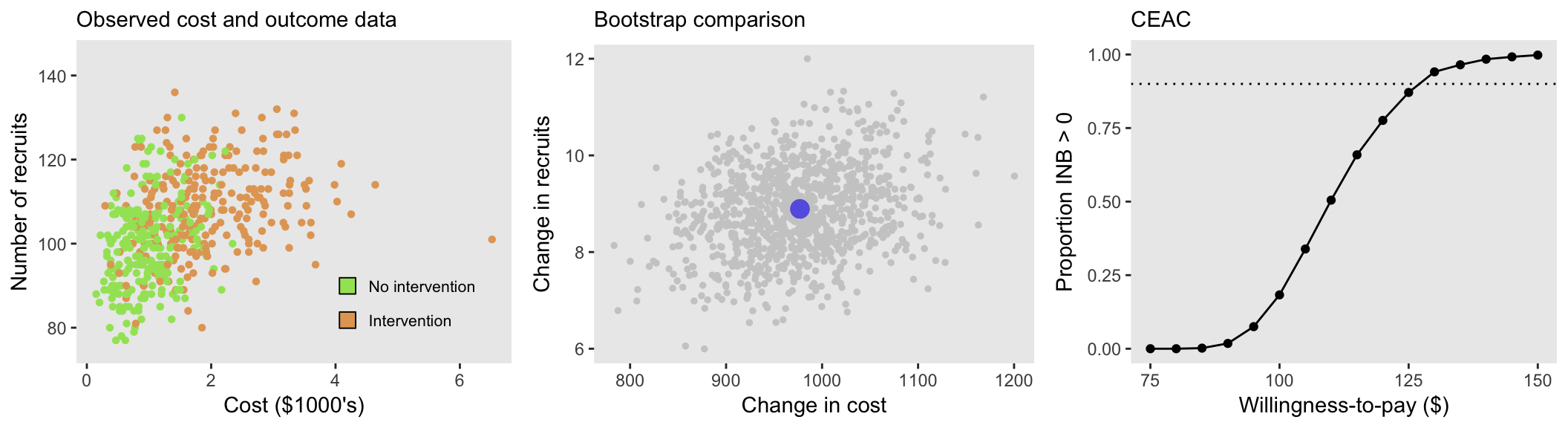
When there is no correlation between costs and recruitment across sites (tau = 0):

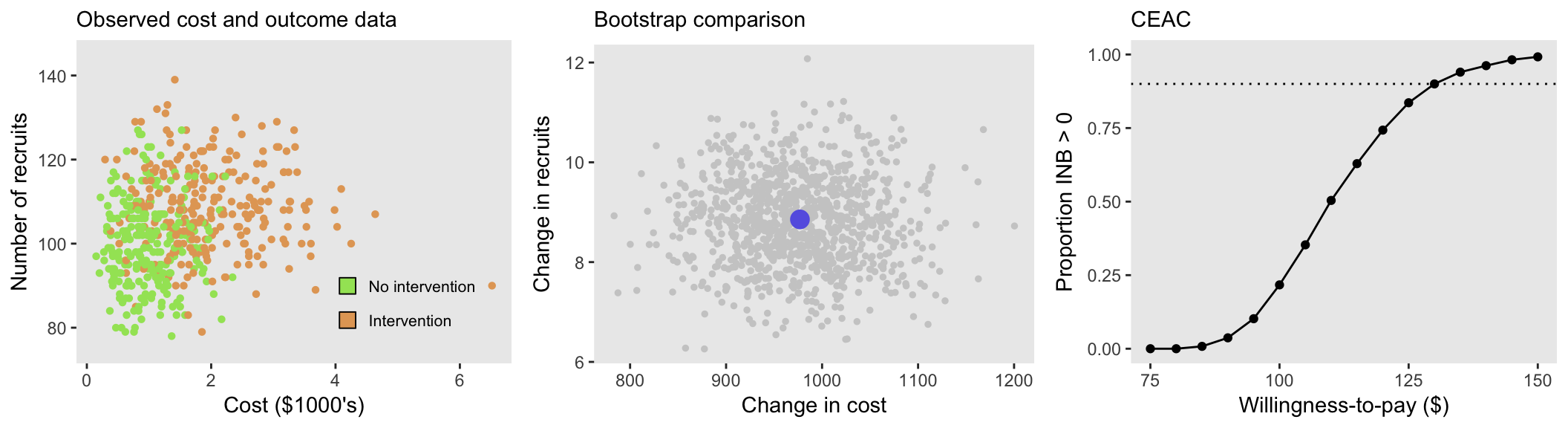
And finally - when there is a higher degree of correlation, tau = 0.4:

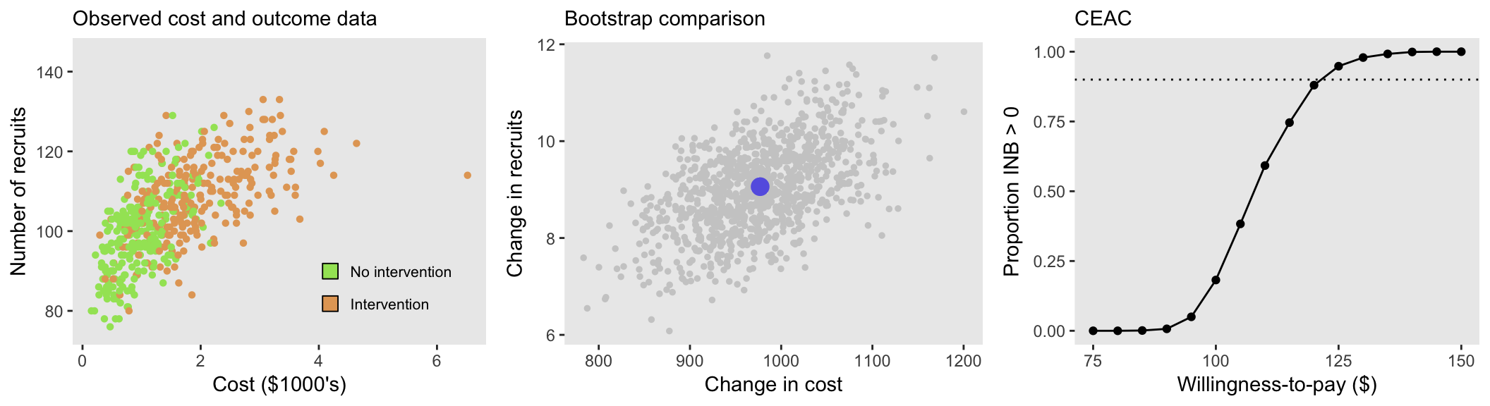
Effect of correlation?

In all three scenarios (with different levels of tau), the ICER is approximately $110. Of course, this is directly related to the fact that the estimated differences in means of the two intervention groups is the same across the scenarios. But, when we look at the three site-level and bootstrap plots, we can see the varying levels of correlation.

And while there also appears to be a subtle visual difference between the CEAC’s for different levels of correlation, it is not clear if this is a real difference or random variation. To explore this a bit further, I generated 250 data sets and their associated CEACs (which in turn are generated by 1000 bootstrap steps eacj) under a range of tau’s, starting with no correlation (tau = 0) up to a considerable level of correlation (tau = 0.4). In these simulations, I used a larger sample size of 2000 sites to reduce the variation a bit. Here are the results:

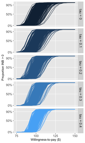
It appears that the variability of the CEAC curves decreases as correlation between cost and recruitment (determined by tau) increases; the range of the curves is smallest when tau is 0.4. In addition, in looks like the “median” CEAC moves slightly rightward as tau increases, which suggests that probability of cost-effectiveness will vary across different levels of tau. All this is to say that correlation appears to matter, so it might be an important factor to consider when both simulating these sorts of data and actually conducting a CEA.

Next steps?

In this example, I based the entire analysis on a simple non-parametric estimate of the means. In the future, I might explore copula-based methods to fit joint models of costs and outcomes. In simstudy, a Gaussian copula generates the correlated data. However there is a much larger world of copulas out there that can be used to model correlation between measures regardless of their marginal distributions. And some of these methods have been applied in the context of CEA. Stay tuned on this front (though it might be a while).