Adding a "mixture" distribution to the simstudy package

Specifying the “mixture” distribution

As defined here, a mixture of variables is a random draw from a set of variables based on a defined set of probabilities. For example, if we have two variables, \(x_1\) and \(x_2\), we have a mixture if, for any particular observation, we take \(x_1\) with probability \(p_1\) and \(x_2\) with probability \(p_2\), where \(\sum_i{p_i} = 1\), \(i \in (1, 2)\). So, if we have already defined \(x_1\) and \(x_2\) using the defData function, we can create a third variable \(x_{mix}\) with this definition:

def <- defData(def, varname = "xMix", 
               formula = "x1 | 0.4 + x2 | 0.6", 
               dist = "mixture")

In this example, we will draw \(x_1\) with probability 0.4 and \(x_2\) with probability 0.6. We are, however, not limited to mixing only two variables; to make that clear, I’ll start off with an example that shows a mixture of three normally distributed variables.

Mixture of 3 normal distributions

In this case, we have \(x_1 \sim N(1,1)\), \(x_2 \sim N(5,4)\), and \(x_3 \sim N(9,1)\). The mixture will draw from \(x_1\) 30% of the time, from \(x_2\) 40%, and from \(x_3\) 30%:

def <- defData(varname = "x1", formula = 1, variance = 1)
def <- defData(def, varname = "x2", formula = 5, variance = 4)
def <- defData(def, varname = "x3", formula = 9, variance = 1)
def <- defData(def, varname = "xMix", 
               formula = "x1 | .3 + x2 | .4 + x3 | .3", 
               dist = "mixture")

The data generation now proceeds as usual in simstudy:

set.seed(2716)
dx <- genData(1000, def)
dx

##         id     x1   x2    x3   xMix
##    1:    1  1.640 4.12  7.13  4.125
##    2:    2 -0.633 6.89  9.07 -0.633
##    3:    3  1.152 2.95  8.71  1.152
##    4:    4  1.519 5.53  8.82  5.530
##    5:    5  0.206 5.55  9.31  5.547
##   ---                              
##  996:  996  2.658 1.87  8.09  1.870
##  997:  997  2.604 4.44  9.09  2.604
##  998:  998  0.457 5.56 10.87 10.867
##  999:  999 -0.400 4.29  9.03 -0.400
## 1000: 1000  2.838 4.78  9.17  9.174

Here are two plots. The top shows the densities for the original distributions separately, and the bottom plot shows the mixture distribution (which is the distribution of xMix):

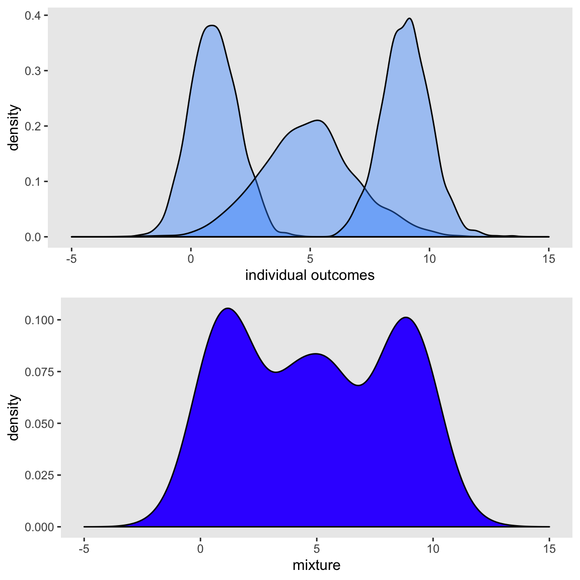
And it is easy to show that the mixture proportions are indeed based on the probabilities that were defined:

dx[, .(p1=mean(xMix == x1), p2=mean(xMix == x2), p3=mean(xMix == x3))]

##       p1    p2    p3
## 1: 0.298 0.405 0.297

Zero-inflated

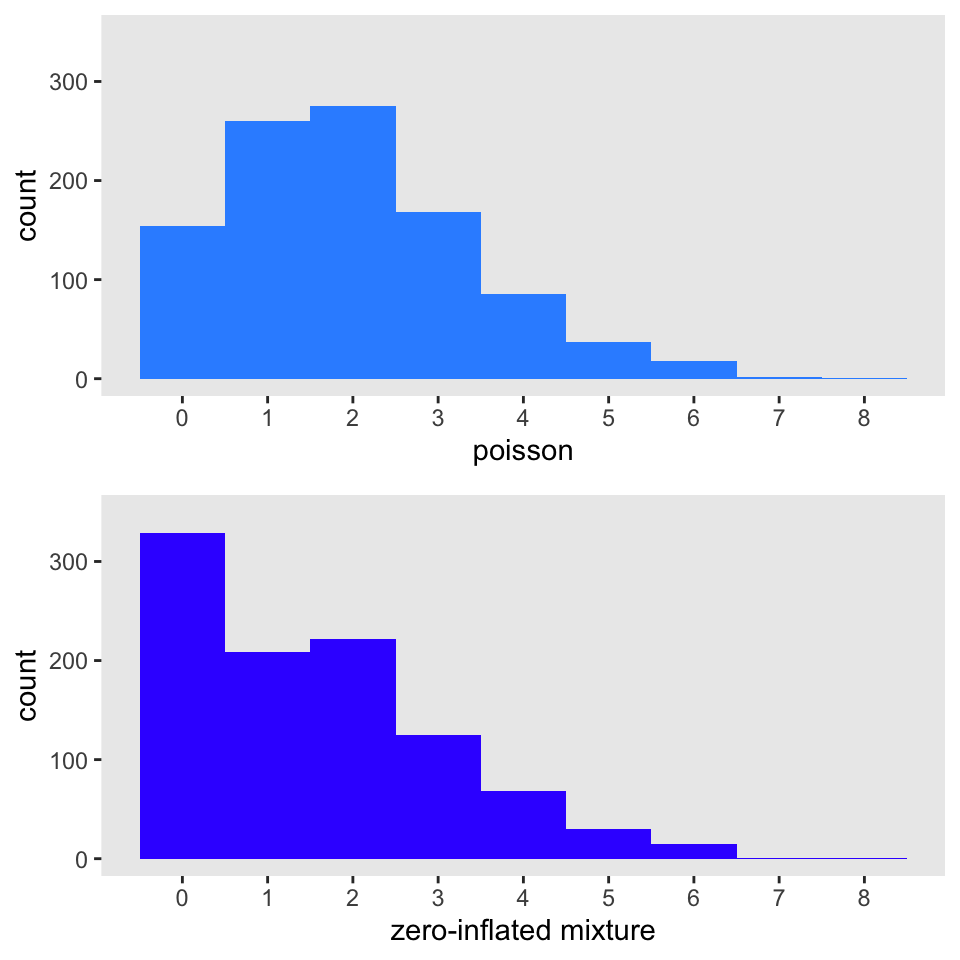
One classic mixture model is the zero-inflated Poisson model. We can easily generate data from this model using a mixture distribution. In this case, the outcome is \(0\) with probability \(p\) and is a draw from a Poisson distribution with mean (and variance) \(\lambda\) with probability \(1-p\). As a result, there will be an over-representation of 0’s in the observed data set. In this example \(p\) = 0.2 and \(\lambda = 2\):

def <- defData(varname = "x0", formula = 0, dist = "nonrandom")
def <- defData(def, varname = "xPois", formula = 2, dist = "poisson")
def <- defData(def, varname = "xMix", formula = "x0 | .2 + xPois | .8", 
               dist = "mixture")

set.seed(2716)
dx <- genData(1000, def)

The figure below shows a histogram of the Poisson distributed \(x_{pois}\) on top and a histogram of the mixture on the bottom. It is readily apparent that the mixture distribution has “too many” zeros relative to the Poisson distribution:

I am fitting model below (using the pscl package) to see if it is possible to recover the assumptions I used in the data generation process. With 1000 observations, of course, it is easy:

library(pscl)
zfit <- zeroinfl(xMix ~ 1 | 1, data = dx)

summary(zfit)

## 
## Call:
## zeroinfl(formula = xMix ~ 1 | 1, data = dx)
## 
## Pearson residuals:
##    Min     1Q Median     3Q    Max 
## -1.035 -1.035 -0.370  0.296  4.291 
## 
## Count model coefficients (poisson with log link):
##             Estimate Std. Error z value Pr(>|z|)    
## (Intercept)   0.6959     0.0306    22.8   <2e-16 ***
## 
## Zero-inflation model coefficients (binomial with logit link):
##             Estimate Std. Error z value Pr(>|z|)    
## (Intercept)   -1.239      0.107   -11.5   <2e-16 ***
## ---
## Signif. codes:  0 '***' 0.001 '**' 0.01 '*' 0.05 '.' 0.1 ' ' 1 
## 
## Number of iterations in BFGS optimization: 9 
## Log-likelihood: -1.66e+03 on 2 Df

The estimated value of \(lambda\) from the model is the exponentiated value of the coefficient from the Poisson model: \(e^{0.6959}\). The estimate is quite close to the true value \(\lambda = 2\):

exp(coef(zfit)[1])

## count_(Intercept) 
##              2.01

And the estimated probability of drawing a zero (i.e. \(\hat{p}\)) is based on a simple transformation of the coefficient of the binomial model (\(-1.239\)), which is on the logit scale. Again, the estimate is quite close to the true value \(p = 0.2\):

1/(1 + exp(-coef(zfit)[2]))

## zero_(Intercept) 
##            0.225

Outlier in linear regression

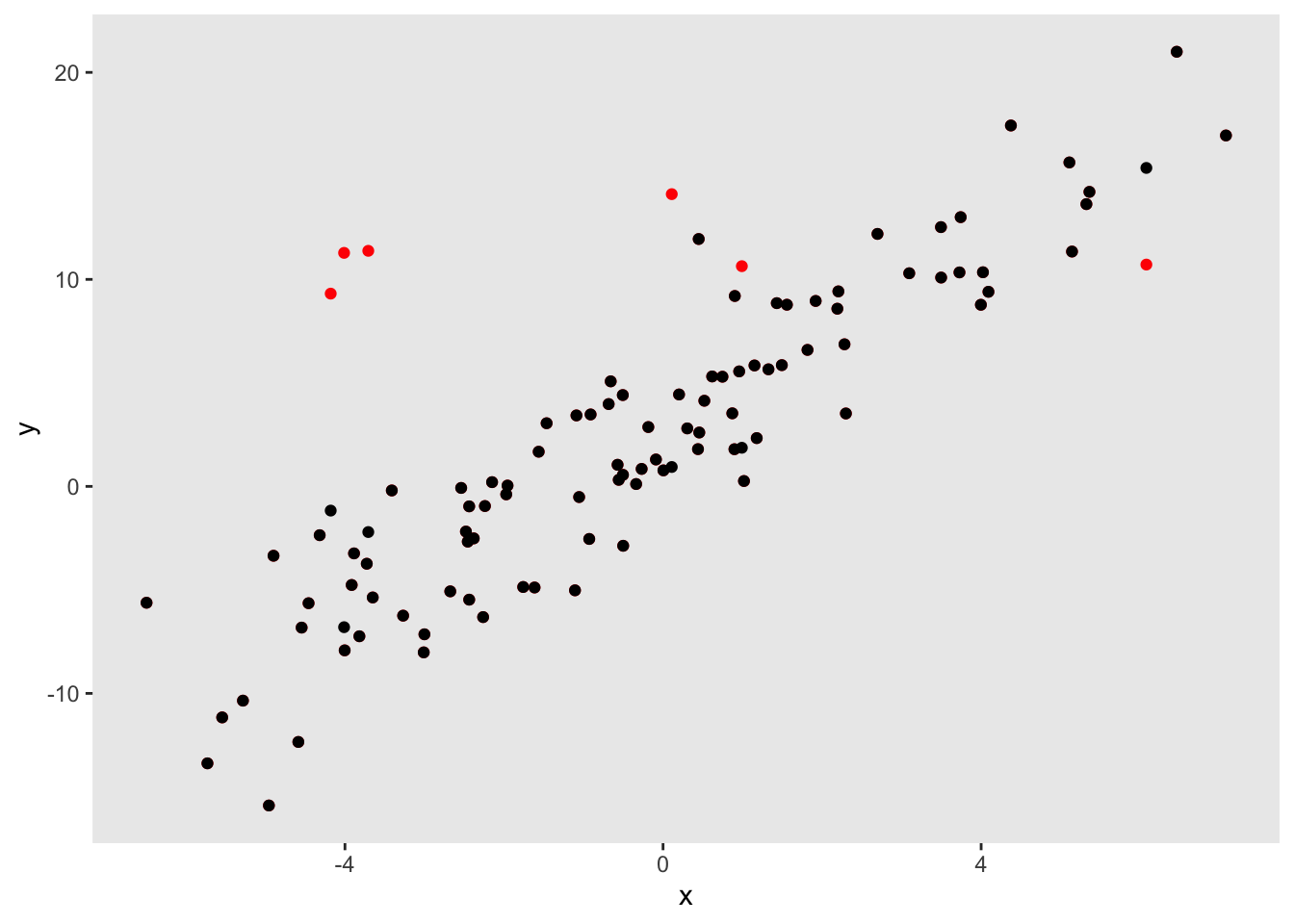
In this final example, I use the mixture option to generate outliers in the context of a regression model. This is done first by generating outcomes \(y\) as a function of a predictor \(x\). Next, alternative outcomes \(y_{outlier}\) are generated independent of \(x\). The observed outcomes \(y_{obs}\) are a mixture of the outliers \(y_{outlier}\) and the predicted \(y\)’s. In this simulation, 2.5% of the observations will be drawn from the outliers:

def <- defData(varname = "x", formula = 0, variance = 9, 
               dist = "normal")
def <- defData(def, varname = "y", formula = "3+2*x", variance = 7, 
               dist = "normal")
def <- defData(def, varname = "yOutlier", formula = 12, variance = 6, 
               dist = "normal")
def <- defData(def, varname = "yObs", 
               formula = "y | .975 + yOutlier | .025", 
               dist = "mixture")

set.seed(2716)
dx <- genData(100, def)

This scatter plot shows the relationship between \(y_{obs}\) and \(x\); the red dots represent the observations drawn from the outlier distribution:

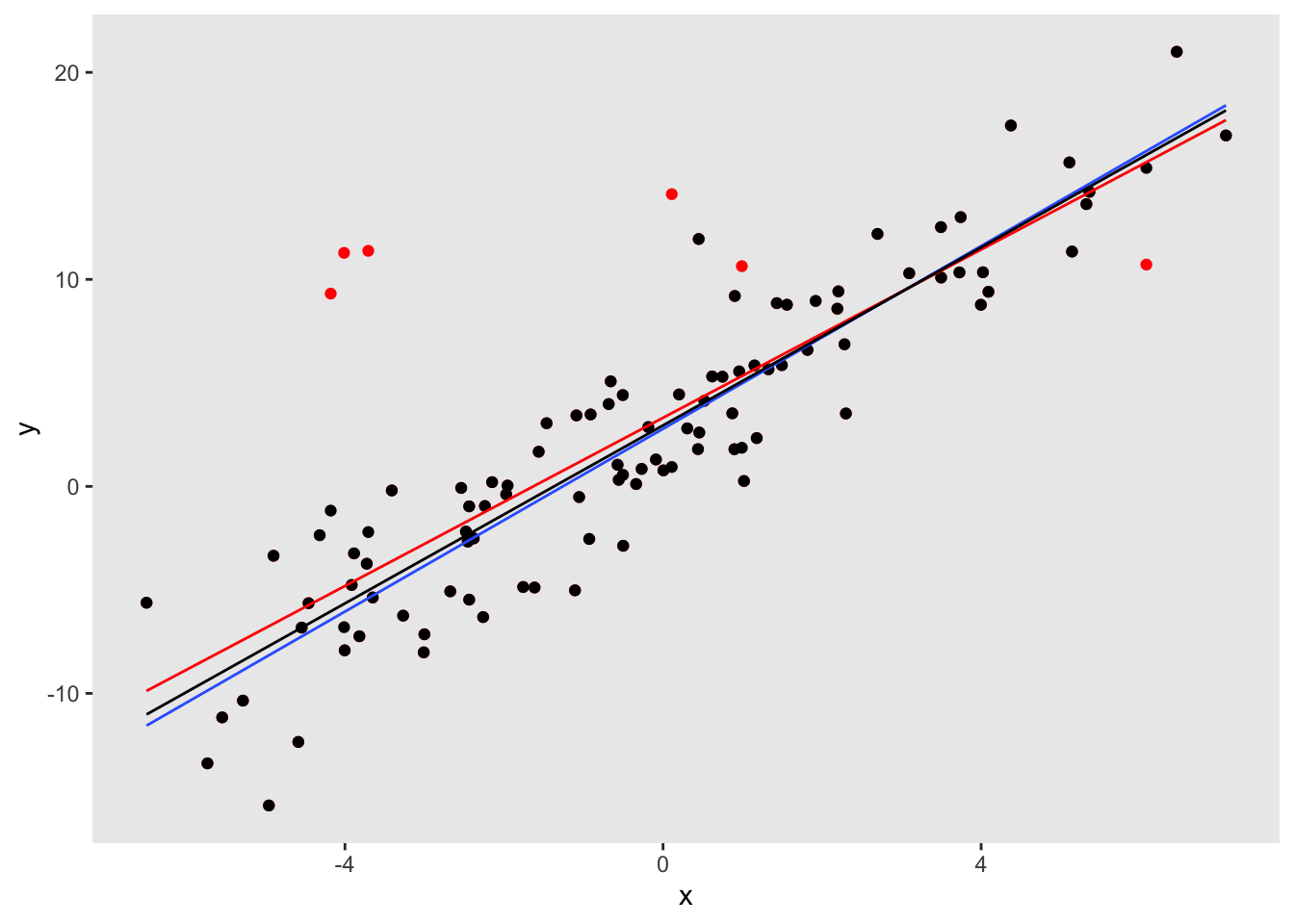
Once again, it is illustrative to fit a few models to estimate the linear relationships between the \(y\) and \(x\). The model that includes the true value of \(y\) (as opposed to the outliers) unsurprisingly recovers the true relationship. The model that includes the observed outcomes (the mixture distribution) underestimates the relationship. And a robust regression model (using the rlm function MASS package) provides a less biased estimate:

lm1 <- lm( y ~ x, data = dx)
lm2 <- lm( yObs ~ x, data = dx)

library(MASS)
rr <- rlm(yObs ~ x , data = dx)

library(stargazer)

stargazer(lm1, lm2, rr, type = "text",
          omit.stat = "all", omit.table.layout = "-asn",
          report = "vcs")

## 
## ================================
##            Dependent variable:  
##          -----------------------
##             y         yObs      
##            OLS     OLS   robust 
##                          linear 
##            (1)     (2)     (3)  
## x         2.210   2.030   2.150 
##          (0.093) (0.136) (0.111)
##                                 
## Constant  2.780   3.310   2.950 
##          (0.285) (0.417) (0.341)
##                                 
## ================================

The scatter plot below includes the fitted lines from the estimated models: the blue line is the true regression model, the red line is the biased estimate based on the data that includes outliers, and the black line is the robust regression line that is much closer to the truth:

The mixture option is still experimental, though it is available on github. One enhancement I hope to make is to allow the mixture probability to be a function of covariates. The next release on CRAN will certainly include some form of this new distribution option.