This is a relatively brief addendum to last week’s post, where I described how the rvar datatype implemented in the R package posterior makes it quite easy to perform posterior probability checks to assess goodness of fit. In the initial post, I generated data from a linear model and estimated parameters for a linear regression model, and, unsurprisingly, the model fit the data quite well. When I introduced a quadratic term into the data generating process and fit the same linear model (without a quadratic term), equally unsurprising, the model wasn’t a great fit.
Immediately after putting the post up, I decided to make sure the correct model with the quadratic term would not result in extreme p-value (i.e. would fall between 0.02 and 0.98). And, again not surprisingly, the model was a good fit. I’m sharing all this here, because I got some advice on how to work with the rvar data a little more efficiently, and wanted to make sure those who are interested could see that. And while I was at it, I decided to investigate the distribution of Bayesian p-values under the condition that the model and data generating process are the same (i.e. the model is correct).
Just as a reminder, here is the data generation process:
\[y \sim N(\mu = 2 + 6*x - 0.3x^2, \ \sigma^2 = 4)\]
Here are the necessary libraries:
library(simstudy)
library(data.table)
library(cmdstanr)
library(posterior)
library(bayesplot)
library(ggplot2)
And here is the data generation:
b_quad <- -0.3

ddef <- defData(varname = "x", formula = "0;10", dist = "uniform")
ddef <- defData(ddef, "y", "2 + 6*x + ..b_quad*(x^2)", 4)

set.seed(72612)
dd <- genData(100, ddef)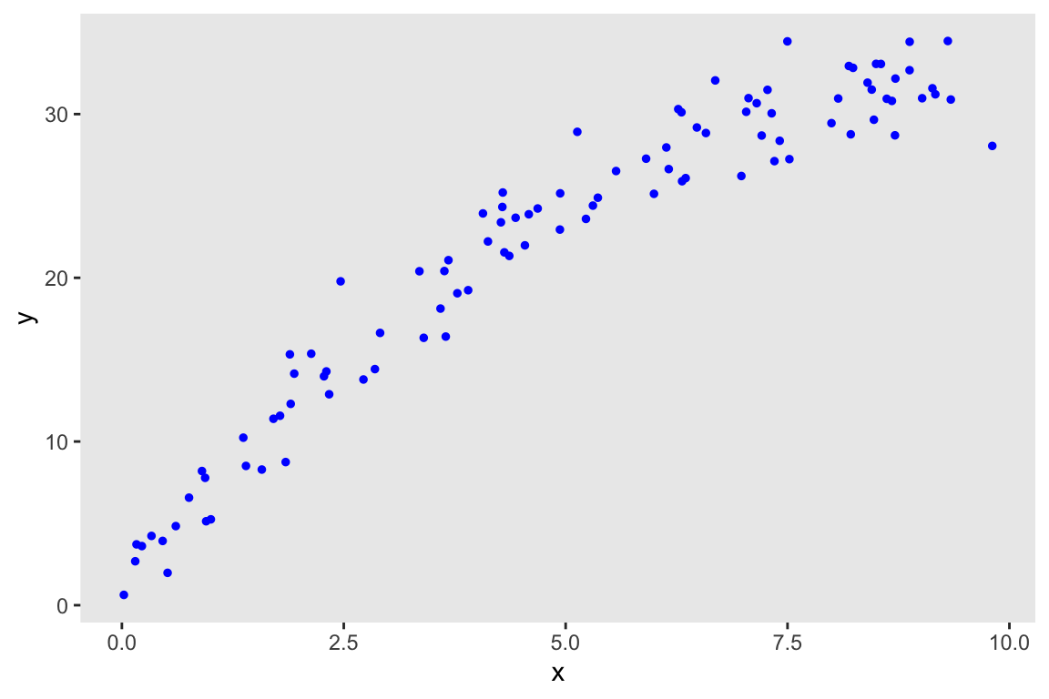
The Stan model is slightly modified to include the additional term; \(\gamma\) is the quadratic parameter:
data {
  int<lower=0> N;
  vector[N] x;
  vector[N] y;
}

transformed data{
  vector[N] x2;

  for (i in 1:N) {
    x2[i] = x[i]*x[i];
  };

}

parameters {
  real alpha;
  real beta;
  real gamma;
  real<lower=0> sigma;
}

model {
  y ~ normal(alpha + beta*x + gamma*x2, sigma);
}
mod <- cmdstan_model("code/quadratic_regression.stan")fit <- mod$sample(
data = list(N = nrow(dd), x = dd$x, y = dd$y),
seed = 72651,
refresh = 0,
chains = 4L,
parallel_chains = 4L,
iter_warmup = 500,
iter_sampling = 2500
)## Running MCMC with 4 parallel chains...
##
## Chain 3 finished in 0.5 seconds.
## Chain 1 finished in 0.5 seconds.
## Chain 2 finished in 0.5 seconds.
## Chain 4 finished in 0.5 seconds.
##
## All 4 chains finished successfully.
## Mean chain execution time: 0.5 seconds.
## Total execution time: 0.6 seconds.As before, I am plotting the observed (actual data) along with the 80% intervals of predicted values at each level of \(x\). The observed data appear to be randomly scattered within the intervals with no apparent pattern:
post_rvars <- as_draws_rvars(fit$draws())

mu <- with(post_rvars, alpha + beta * as_rvar(dd$x) + gamma * as_rvar(dd$x^2))
pred <- rvar_rng(rnorm, nrow(dd), mu, post_rvars$sigma)

df.80 <- data.table(x = dd$x, y=dd$y, t(quantile(pred, c(0.10, 0.90))))
df.80[, extreme := !(y >= V1 & y <= V2)]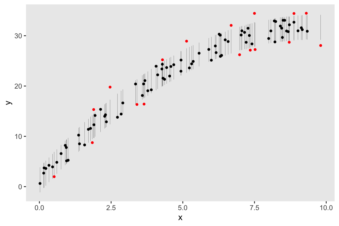
The code to estimate the p-value is slightly modified from last time. The important difference is that the lists of rvars (bin_prop_y and bin_prop_pred) are converted directly into vectors of rvars using the do.call function:
df <- data.frame(x = dd$x, y = dd$y, mu, pred)
df$grp <- cut(df$x, breaks = seq(0, 10, by = 2),include.lowest = TRUE, labels=FALSE)
bin_prop_y <- lapply(split(df, df$grp), function(x) rvar_mean(x$y < x$mu))
rv_y <- do.call(c, bin_prop_y)
T_y <- rvar_var(rv_y)
bin_prop_pred <- lapply(split(df, df$grp), function(x) rvar_mean(x$pred < x$mu))
rv_pred <- do.call(c, bin_prop_pred)
T_pred <- rvar_var(rv_pred)
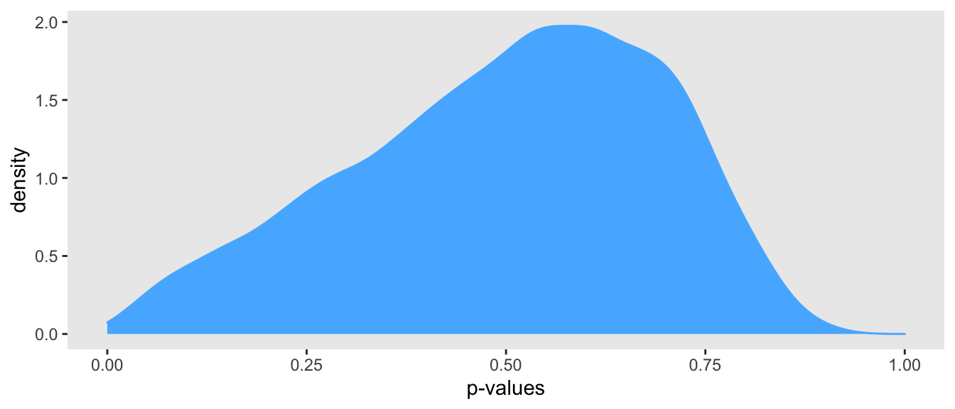
mean(T_pred > T_y)## [1] 0.583In this one case, the p-value is 0.58, suggesting the model is a good fit. But, could this have been a fluke? Looking below at the density plot of p-values based on 10,000 simulated data sets suggests not; indeed, \(P(0.02 < \text{p-value} < 0.98) = 99.8\%.\) (If you are interested in the code that estimated the density of p-values, I can post it as well.)