Recently, we were planning a study to evaluate the effect of an intervention on outcomes for very sick patients who show up in the emergency department. My collaborator had concerns about a phenomenon that she had observed in other studies that might affect the results - patients measured earlier in the study tend to be sicker than those measured later in the study. This might not be a problem, but in the context of a stepped-wedge study design (see this for a discussion that touches this type of study design), this could definitely generate biased estimates: when the intervention occurs later in the study (as it does in a stepped-wedge design), the “exposed” and “unexposed” populations could differ, and in turn so could the outcomes. We might confuse an artificial effect as an intervention effect.
What could explain this phenomenon? The title of this post provides a hint: cases earlier in a study are more likely to be prevalent ones (i.e. they have been sick for a while), whereas later in the study cases tend to be incident (i.e. they only recently become sick). Even though both prevalent and incident cases are sick, the former may be sicker on average than the latter, simply because their condition has had more time develop.
We didn’t have any data to test out this hypothesis (if our grant proposal is funded, we will be able to do that), so I decided to see if I could simulate this phenomenon. In my continuing series exploring simulation using Rcpp, simstudy, and data.table, I am presenting some code that I used to do this.
Generating a population of patients
The first task is to generate a population of individuals, each of whom starts out healthy and potentially becomes sicker over time. Time starts in month 1 and ends at some fixed point - in the first example, I end at 400 months. Each individual has a starting health status and a start month. In the examples that follow, health status is 1 through 4, with 1 being healthy, 3 is quite sick, and 4 is death. And, you can think of the start month as the point where the individual ages into the study. (For example, if the study includes only people 65 and over, the start month is the month the individual turns 65.) If an individual starts in month 300, she will have no measurements in periods 1 through 299 (i.e. health status will be 0).
The first part of the simulation generates a start month and starting health status for each individual, and then generates a health status for each individual until the end of time. Some individuals may die, while others may go all the way to the end of the simulation in a healthy state.
Rcpp function to generate health status for each period
While it is generally preferable to avoid loops in R, sometimes it cannot be avoided. I believe generating a health status that depends on the previous health status (a Markov process) is one of those situations. So, I have written an Rcpp function to do this - it is orders of magnitude faster than doing this in R:
#include <RcppArmadilloExtensions/sample.h>
// [[Rcpp::depends(RcppArmadillo)]]

using namespace Rcpp;

// [[Rcpp::export]]
IntegerVector MCsim( unsigned int nMonths, NumericMatrix P,
                     int startStatus, unsigned int startMonth ) {

  IntegerVector sim( nMonths );
  IntegerVector healthStats( P.ncol() );
  NumericVector currentP;
  IntegerVector newstate;

  unsigned int q = P.ncol();
  healthStats = Rcpp::seq(1, q);

  sim[startMonth - 1] = startStatus;

  /* Loop through each month for each individual */

  for (unsigned int i = startMonth; i < nMonths; i++) {

    /* new state based on health status of last period and
       probability of transitioning to different state     */

    newstate = RcppArmadillo::sample( healthStats,
                                      1,
                                      TRUE,
                                      P.row(sim(i-1) - 1) );
    sim(i) = newstate(0);

  }

  return sim;
}
Generating the data
The data generation process is shown below. The general outline of the process is (1) define transition probabilities, (2) define starting health status distribution, (3) generate starting health statuses and start months, and (4) generate health statuses for each follow-up month.
# Transition matrix for moving through health statuses

P <- matrix(c(0.985, 0.015, 0.000, 0.000,
              0.000, 0.950, 0.050, 0.000,
              0.000, 0.000, 0.850, 0.150,
              0.000, 0.000, 0.000, 1.000), nrow = 4, byrow = TRUE)

maxFU = 400
nPerMonth = 350
N = maxFU * nPerMonth

ddef <- defData(varname = "sHealth",
                formula = "0.80; 0.15; 0.05",
                dist = "categorical")

# generate starting health values (1, 2, or 3) for all individuals
set.seed(123)
did <- genData(n = N, dtDefs = ddef)

# each month, 350 age in to the sample
did[, sMonth := rep(1:maxFU, each = nPerMonth)]

# show table for 10 randomly selected individuals
did[id %in% sample(x = did$id, size = 10, replace = FALSE)]
## id sHealth sMonth
## 1: 15343 2 44
## 2: 19422 2 56
## 3: 41426 1 119
## 4: 50050 1 143
## 5: 63042 1 181
## 6: 83584 1 239
## 7: 93295 1 267
## 8: 110034 1 315
## 9: 112164 3 321
## 10: 123223 1 353# generate the health status history based on the transition matrix
dhealth <- did[, .(sHealth, sMonth, health = MCsim(maxFU, P, sHealth, sMonth)),
keyby = id]
dhealth[, month := c(1:.N), by = id]
dhealth## id sHealth sMonth health month
## 1: 1 1 1 1 1
## 2: 1 1 1 1 2
## 3: 1 1 1 1 3
## 4: 1 1 1 1 4
## 5: 1 1 1 1 5
## ---
## 55999996: 140000 1 400 0 396
## 55999997: 140000 1 400 0 397
## 55999998: 140000 1 400 0 398
## 55999999: 140000 1 400 0 399
## 56000000: 140000 1 400 1 400Simulation needs burn-in period
The simulation process itself is biased in its early phases as there are too many individuals in the sample who have just aged in compared to those who are “older”. (This is sort of the the reverse of the incidence - prevalence bias.) Since individuals tend to have better health status when they are “younger”, the average health status of the simulation in its early phases is biased downwards by the preponderance of young individuals in the population. This suggests that any evaluation of simulated data needs to account for a “burn-in” period that ensures there is a mix of “younger” and “older” individuals. To show this, I have calculated an average health score for each period of the simulation and plotted the results. You can see that the sample stabilizes after about 200 months in this simulation.
# count number of individuals with a particular heath statust each month

cmonth <- dhealth[month > 0, .N, keyby = .(month, health)]
cmonth
## month health N
## 1: 1 0 139650
## 2: 1 1 286
## 3: 1 2 47
## 4: 1 3 17
## 5: 2 0 139300
## ---
## 1994: 399 4 112203
## 1995: 400 1 18610
## 1996: 400 2 6515
## 1997: 400 3 2309
## 1998: 400 4 112566# transform data from "long" form to "wide" form and calculate average
mtotal <- dcast(data = cmonth,
formula = month ~ health,
fill = 0,
value.var = "N")
mtotal[, total := `1` + `2` + `3`]
mtotal[, wavg := (`1` + 2*`2` + 3*`3`)/total]
mtotal## month 0 1 2 3 4 total wavg
## 1: 1 139650 286 47 17 0 350 1.231429
## 2: 2 139300 558 106 32 4 696 1.244253
## 3: 3 138950 829 168 45 8 1042 1.247601
## 4: 4 138600 1104 215 66 15 1385 1.250542
## 5: 5 138250 1362 278 87 23 1727 1.261726
## ---
## 396: 396 1400 18616 6499 2351 111134 27466 1.407813
## 397: 397 1050 18613 6537 2321 111479 27471 1.406938
## 398: 398 700 18587 6561 2323 111829 27471 1.407957
## 399: 399 350 18602 6541 2304 112203 27447 1.406201
## 400: 400 0 18610 6515 2309 112566 27434 1.405810ggplot(data = mtotal, aes(x=month, y=wavg)) +
geom_line() +
ylim(1.2, 1.5) +
geom_hline(yintercept = 1.411, lty = 3) +
geom_vline(xintercept = 200, lty = 3) +
xlab("Month") +
ylab("Average health status") +
theme(panel.background = element_rect(fill = "grey90"),
panel.grid = element_blank(),
plot.title = element_text(size = 12, vjust = 0.5, hjust = 0) ) +
ggtitle("Average health status of simulated population")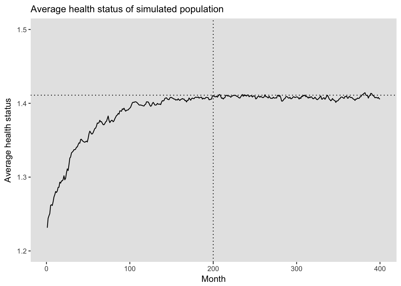
Generating monthly study cohorts
Now we are ready to see if we can simulate the incidence - prevalence bias. The idea here is to find the first month during which an individual (1) is “active” (i.e. the period being considered is on or after the individual’s start period), (2) has an emergency department visit, and (3) whose health status has reached a specified threshold.
We can set a final parameter that looks back some number of months (say 6 or 12) to see if there have been any previous qualifying emergency room visits before the study start period (which in our case will be month 290 to mitigate an burn-in bias identified above). This “look-back” will be used to mitigate some of the bias by creating a washout period that makes the prevalent cases look more like incident cases. This look-back parameter is calculated each month for each individual using an Rcpp function that loops through each period:
#include <Rcpp.h>

using namespace Rcpp;

// [[Rcpp::export]]
IntegerVector cAddPrior(IntegerVector idx,
                        IntegerVector event,
                        int lookback) {

  int nRow = idx.length();
  IntegerVector sumPrior(nRow, NA_INTEGER);

  for (unsigned int i = lookback; i < nRow; i++) {

    IntegerVector seqx = Rcpp::seq(i-lookback, i-1);
    IntegerVector x = event[seqx];
    sumPrior[i] = sum(x);

  }

  return(sumPrior);
}
Generating a single cohort
The following code (1) generates a population (as we did above), (2) generates emergency department visits that are dependent on the health status (the sicker an individual is, the more likely they are to go to the ED), (3) calculates the number of eligible ED visits during the look-back period, and (4) creates the monthly cohorts based on the selection criteria. At the end, we calculate average health status for the cohort by month of cohort - this will be used to illustrate the bias.
maxFU = 325
nPerMonth = 100
N = maxFU * nPerMonth

START = 289 # to allow for adequate burn-in
HEALTH = 2
LOOKBACK = 6 # how far to lookback

set.seed(123)
did <- genData(n = N, dtDefs = ddef)
did[, sMonth := rep(1:maxFU, each = nPerMonth)]

healthStats <- did[, .(sHealth,
                       sMonth,
                       health = MCsim(maxFU, P, sHealth, sMonth)),
                   keyby = id]

healthStats[, month := c(1:.N), by = id]

# eliminate period without status measurement (0) & death (4)
healthStats <- healthStats[!(health %in% c(0,4))]

# ensure burn-in by starting with observations far
# into simulation
healthStats <- healthStats[month > (START - LOOKBACK)]

# set probability of emergency department visit
healthStats[, pED := (health == 1) * 0.02 +
                     (health == 2) * 0.10 +
                     (health == 3) * 0.20]

# generate emergency department visit
healthStats[, ed := rbinom(.N, 1, pED)]

healthStats[, edAdj := ed * as.integer(health >= HEALTH)] # if you want to restrict
healthStats[, pSum := cAddPrior(month, edAdj, lookback = LOOKBACK), keyby=id]

# look at one individual
healthStats[id == 28069]
## id sHealth sMonth health month pED ed edAdj pSum
## 1: 28069 1 281 1 284 0.02 0 0 NA
## 2: 28069 1 281 1 285 0.02 0 0 NA
## 3: 28069 1 281 1 286 0.02 0 0 NA
## 4: 28069 1 281 1 287 0.02 0 0 NA
## 5: 28069 1 281 2 288 0.10 0 0 NA
## 6: 28069 1 281 2 289 0.10 0 0 NA
## 7: 28069 1 281 2 290 0.10 1 1 0
## 8: 28069 1 281 2 291 0.10 0 0 1
## 9: 28069 1 281 2 292 0.10 0 0 1
## 10: 28069 1 281 2 293 0.10 0 0 1
## 11: 28069 1 281 2 294 0.10 0 0 1
## 12: 28069 1 281 3 295 0.20 1 1 1# cohort includes individuals with 1 prior ed visit in
# previous 6 months
cohort <- healthStats[edAdj == 1 & pSum == 0]
cohort <- cohort[, .(month = min(month)), keyby = id]
cohort## id month
## 1: 53 306
## 2: 82 313
## 3: 140 324
## 4: 585 291
## 5: 790 299
## ---
## 3933: 31718 324
## 3934: 31744 325
## 3935: 31810 325
## 3936: 31860 325
## 3937: 31887 325# estimate average health status of monthly cohorts
cohortStats <- healthStats[cohort, on = c("id","month")]
sumStats <- cohortStats[ , .(avghealth = mean(health), n = .N), keyby = month]
head(sumStats)## month avghealth n
## 1: 290 2.248175 137
## 2: 291 2.311765 170
## 3: 292 2.367347 147
## 4: 293 2.291925 161
## 5: 294 2.366906 139
## 6: 295 2.283871 155Exploring bias
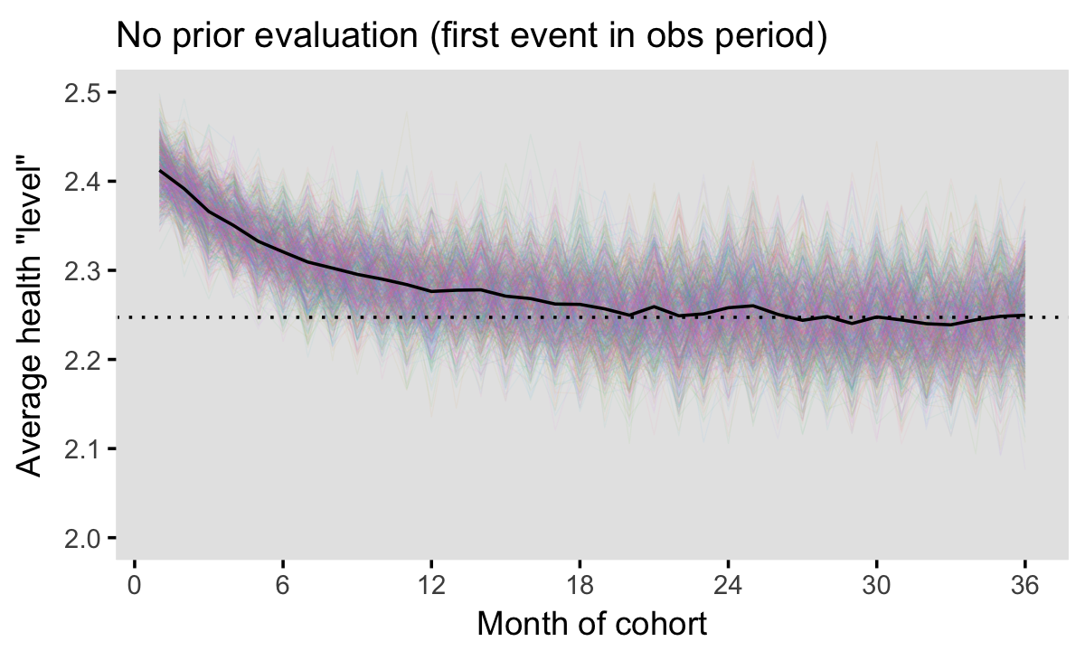
Finally, we are at the point where we can see what, if any, bias results in selecting our cohorts under the scenario I’ve outlined above. We start by generating multiple iterations of populations and cohorts and estimating average health status by month under the assumption that we will have a look-back period of 0. That is, we will accept an individual into the first possible cohort regardless of her previous emergency department visit history. The plot below shows average across 1000 iterations. What we see is that the average health status of the cohorts in the first 20 months or so exceed the long run average. The incidence - prevalence bias is extremely strong if we ignore prior ED history!
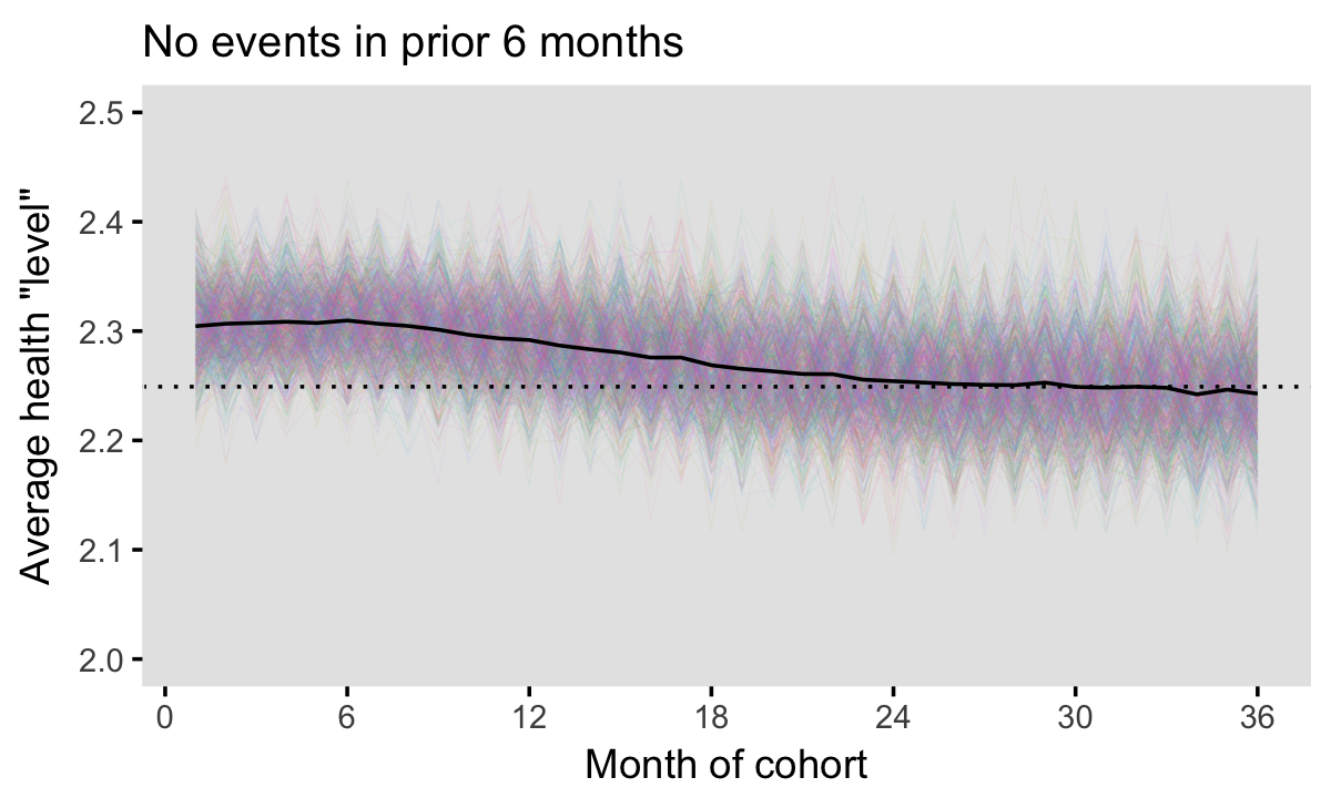
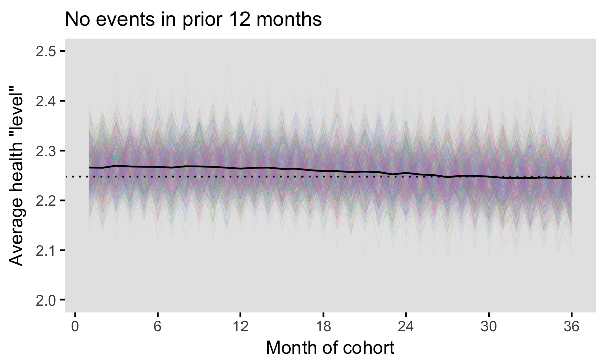
Taking history into account
Once we start to incorporate ED history by using look-back periods greater than 0, we see that we can reduce bias considerably. The two plots below show the results of using look-back periods of 6 and 12 months. Both have reduced bias, but only at 12 months are we approaching something that actually looks desirable. In fact, under this scenario, we’d probably like to go back 24 months to eliminate the bias entirely. Of course, these particular results are dependent on the simulation assumptions, so determining an appropriate look-back period will certainly depend on the actual data. (When we do finally get the actual data, I will follow-up to let you know what kind of adjustment we needed to make in the real, non-simulated world.)