I am involved with a trial of an intervention designed to prevent full-blown opioid use disorder for patients who may have an incipient opioid use problem. Given the nature of the intervention, it was clear the only feasible way to conduct this particular study is to randomize at the physician rather than the patient level.
There was a concern that the number of patients eligible for the study might be limited, so that each physician might only have a handful of patients able to participate, if that many. A question arose as to whether we can make up for this limitation by increasing the number of physicians who participate? That is, what is the trade-off between number of clusters and cluster size?
This is a classic issue that confronts any cluster randomized trial - made more challenging by the potentially very small cluster sizes. A primary concern of the investigators is having sufficient power to estimate an intervention effect - how would this trade-off impact that? And as a statistician, I have concerns about bias and variance, which could have important implications depending on what you are interested in measuring.
Clustering in a nutshell
This is an immense topic - I won’t attempt to point you to the best resources, because there are so many out there. For me, there are two salient features of cluster randomized trials that present key challenges.
First, individuals in a cluster are not providing as much information as we might imagine. If we take an extreme example of a case where the outcome of everyone in a cluster is identical, we learn absolutely nothing by taking an additional subject from that cluster; in fact, all we need is one subject per cluster, because all the variation is across clusters, not within. Of course, that is overly dramatic, but the same principal is in play even when the outcomes of subjects in a cluster are moderately correlated. The impact of this phenomenon depends on the within cluster correlation relative to the between cluster correlation. The relationship of these two correlations is traditionally characterized by the intra-class coefficient (ICC), which is the ratio of the between-cluster variation to total variation.
Second, if there is high variability across clusters, that gets propagated to the variance of the estimate of the treatment effect. From study to study (which is what we are conceiving of in a frequentist frame of mind), we are not just sampling individuals from the clusters, but we are changing the sample of clusters that we are selecting from! So much variation going on. Of course, if all clusters are exactly the same (i.e. no variation between clusters), then it doesn’t really matter what clusters we are choosing from each time around, and we have no added variability as a result of sampling from different clusters. But, as we relax this assumption of no between-cluster variability, we add over-all variability to the process, which gets translated to our parameter estimates.
The cluster size/cluster number trade-off is driven largely by these two issues.
Simulation
I am generating data from a cluster randomized trial that has the following underlying data generating process:
\[ Y_{ij} = 0.35 * R_j + c_j + \epsilon_{ij}\ ,\] where \(Y_{ij}\) is the outcome for patient \(i\) who is being treated by physician \(j\). \(R_j\) represents the treatment indicator for physician \(j\) (0 for control, 1 for treatment). \(c_j\) is the physician-level random effect that is normally distributed \(N(0, \sigma^2_c)\). \(\epsilon_{ij}\) is the individual-level effect, and \(\epsilon_{ij} \sim N(0, \sigma^2_\epsilon)\). The expected value of \(Y_{ij}\) for patients treated by physicians in the control group is \(0\). And for the patients treated by physicians in the intervention \(E(Y_{ij}) = 0.35\).
Defining the simulation
The entire premise of this post is that we have a target number of study subjects (which in the real world example was set at 480), and the question is should we spread those subjects across a smaller or larger number of clusters? In all the simulations that follow, then, we have fixed the total number of subjects at 480. That means if we have 240 clusters, there will be only 2 in each one; and if we have 10 clusters, there will be 48 patients per cluster.
In the first example shown here, we are assuming an ICC = 0.10 and 60 clusters of 8 subjects each:
library(simstudy)
Var <- iccRE(0.10, varWithin = 0.90, dist = "normal")

defC <- defData(varname = "ceffect", formula = 0, variance = Var,
                  dist = "normal", id = "cid")
defC <- defData(defC, "nperc", formula = "8",
                  dist = "nonrandom" )

defI <- defDataAdd(varname = "y", formula = "ceffect + 0.35 * rx",
                   variance = 0.90)
Generating a single data set and estimating parameters
Based on the data definitions, I can now generate a single data set:
set.seed(711216)

dc <- genData(60, defC)
dc <- trtAssign(dc, 2, grpName = "rx")

dd <- genCluster(dc, "cid", numIndsVar = "nperc", level1ID = "id" )
dd <- addColumns(defI, dd)

dd
## cid rx ceffect nperc id y
## 1: 1 0 0.71732 8 1 0.42
## 2: 1 0 0.71732 8 2 0.90
## 3: 1 0 0.71732 8 3 -1.24
## 4: 1 0 0.71732 8 4 2.37
## 5: 1 0 0.71732 8 5 0.71
## ---
## 476: 60 1 -0.00034 8 476 -1.12
## 477: 60 1 -0.00034 8 477 0.88
## 478: 60 1 -0.00034 8 478 0.47
## 479: 60 1 -0.00034 8 479 0.28
## 480: 60 1 -0.00034 8 480 -0.54We use a linear mixed effect model to estimate the treatment effect and variation across clusters:
library(lmerTest)
lmerfit <- lmer(y~rx + (1 | cid), data = dd)
Here are the estimates of the random and fixed effects:
as.data.table(VarCorr(lmerfit))## grp var1 var2 vcov sdcor
## 1: cid (Intercept) <NA> 0.14 0.38
## 2: Residual <NA> <NA> 0.78 0.88coef(summary(lmerfit))## Estimate Std. Error df t value Pr(>|t|)
## (Intercept) 0.008 0.089 58 0.09 0.929
## rx 0.322 0.126 58 2.54 0.014And here is the estimated ICC, which happens to be close to the “true” ICC of 0.10 (which is definitely not a sure thing given the relatively small sample size):
library(sjstats)
icc(lmerfit)
##
## Intraclass Correlation Coefficient for Linear mixed model
##
## Family : gaussian (identity)
## Formula: y ~ rx + (1 | cid)
##
## ICC (cid): 0.1540A deeper look at the variation of estimates
In these simulations, we are primarily interested in investigating the effect of different numbers of clusters and different cluster sizes on power, variation, bias (and mean square error, which is a combined measure of variance and bias). This means replicating many data sets and studying the distribution of the estimates.
To do this, it is helpful to create a functions that generates the data:
reps <- function(nclust) {

    dc <- genData(nclust, defC)
    dc <- trtAssign(dc, 2, grpName = "rx")

    dd <- genCluster(dc, "cid", numIndsVar = "nperc", level1ID = "id" )
    dd <- addColumns(defI, dd)

    lmerTest::lmer(y ~ rx + (1 | cid), data = dd)
}
And here is a function to check if p-values from model estimates are less than 0.05, which will come in handy later when estimating power:
pval <- function(x) {
    coef(summary(x))["rx", "Pr(>|t|)"] < 0.05
}
Now we can generate 1000 data sets and fit a linear fixed effects model to each one, and store the results in an R list:
library(parallel)

res <- mclapply(1:1000, function(x) reps(60))
Extracting information from all 1000 model fits provides an estimate of power:
mean(sapply(res, function(x) pval(x)))## [1] 0.82And here are estimates of bias, variance, and root mean square error of the treatment effect estimates. We can see in this case, the estimated treatment effect is not particularly biased:
RX <- sapply(res, function(x) getME(x, "fixef")["rx"])

c(true = 0.35, avg = mean(RX), var = var(RX),
  bias = mean(RX - 0.35), rmse = sqrt(mean((RX - 0.35)^2)))
## true avg var bias rmse
## 0.35000 0.35061 0.01489 0.00061 0.12197And if we are interested in seeing how well we measure the between cluster variation, we can evaluate that as well. The true variance (used to generate the data), was 0.10, and the average of the estimates was 0.099, quite close:
RE <- sapply(res, function(x) as.numeric(VarCorr(x)))

c(true = Var, avg = mean(RE), var = var(RE),
  bias = mean(RE - Var), rmse = sqrt(mean((RE - Var)^2)))
## true avg var bias rmse
## 0.10000 0.10011 0.00160 0.00011 0.03996Replications under different scenarios
Now we are ready to put all of this together for one final experiment to investigate the effects of the ICC and cluster number/size on power, variance, and bias. I generated 2000 data sets for each combination of assumptions about cluster sizes (ranging from 10 to 240) and ICC’s (ranging from 0 to 0.15). For each combination, I estimated the variance and bias for the treatment effect parameter estimates and the between-cluster variance. (I include the code in case any one needs to do something similar.)
ps <- list()
pn <- 0

nclust <- c(10, 20, 30, 40, 48, 60, 80, 96, 120, 160, 240)
iccs <- c(0, 0.02, 0.05 , 0.10, 0.15)

for (s in seq_along(nclust)) {
  for (i in seq_along(iccs)) {

    newvar <- iccRE(iccs[i], varWithin = .90, dist = "normal")
    newperc <- 480/nclust[s]

    defC <- updateDef(defC, "ceffect", newvariance = newvar)
    defC <- updateDef(defC, "nperc", newformula = newperc)

    res <- mclapply(1:2000, function(x) reps(nclust[s]))
    RX <- sapply(res, function(x) getME(x, "fixef")["rx"])
    RE <- sapply(res, function(x) as.numeric(VarCorr(x)))
    power <- mean(sapply(res, function(x) pval(x)))

    pn <- pn + 1
    ps[[pn]] <- data.table(nclust = nclust[s],
                           newperc,
                           icc=iccs[i],
                           newvar,
                           power,
                           biasRX = mean(RX - 0.35),
                           varRX = var(RX),
                           rmseRX = sqrt(mean((RX - 0.35)^2)),
                           avgRE = mean(RE),
                           biasRE = mean(RE - newvar),
                           varRE = var(RE),
                           rmseRE = sqrt(mean((RE - newvar)^2))
    )
  }
}

ps <- data.table::rbindlist(ps)
First, we can take a look at the power. Clearly, for lower ICC’s, there is little marginal gain after a threshold between 60 and 80 clusters; with the higher ICC’s, a study might benefit with respect to power from adding more clusters (and reducing cluster size):
library(ggthemes) # for Paul Tol's Color Schemes
library(scales)

ggplot(data = ps, aes(x = nclust, y = power, group = icc)) +
  geom_smooth(aes(color = factor(icc)), se = FALSE) +
  theme(panel.grid.minor = element_blank()) +
  scale_color_ptol(name = "ICC", labels = number(iccs, accuracy = .01)) +
  scale_x_continuous(name = "number of clusters", breaks = nclust)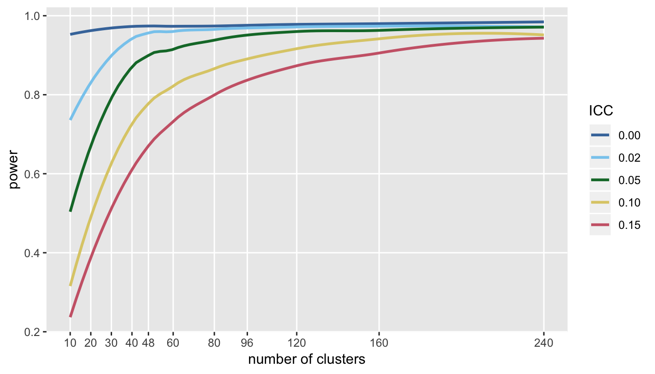
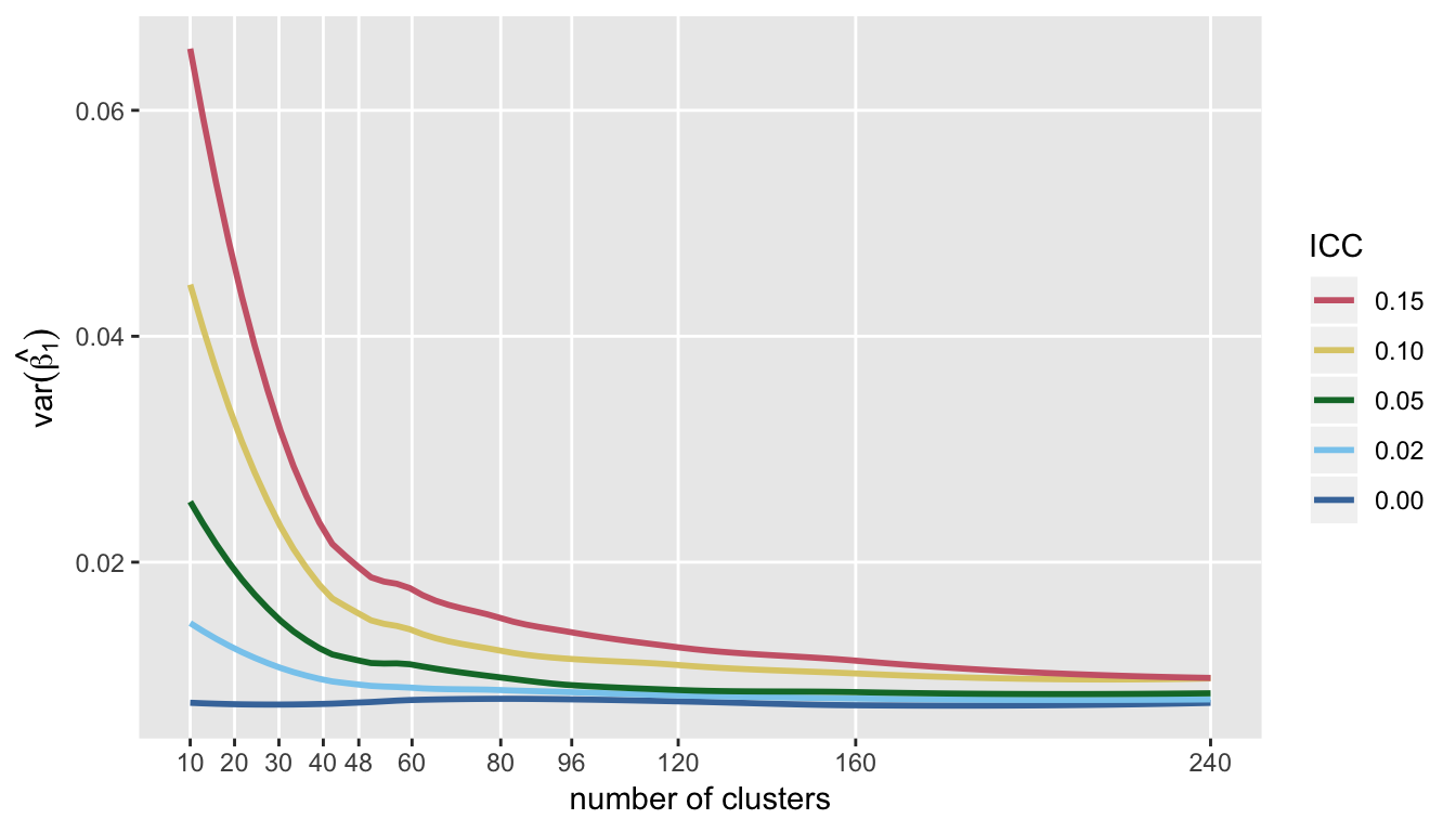
Not surprisingly, the same picture emerges (only in reverse) when looking at the variance of the estimate for treatment effect. Variance declines quite dramatically as we increase the number of clusters (again, reducing cluster size) up to about 60 or so, and little gain in precision beyond that:
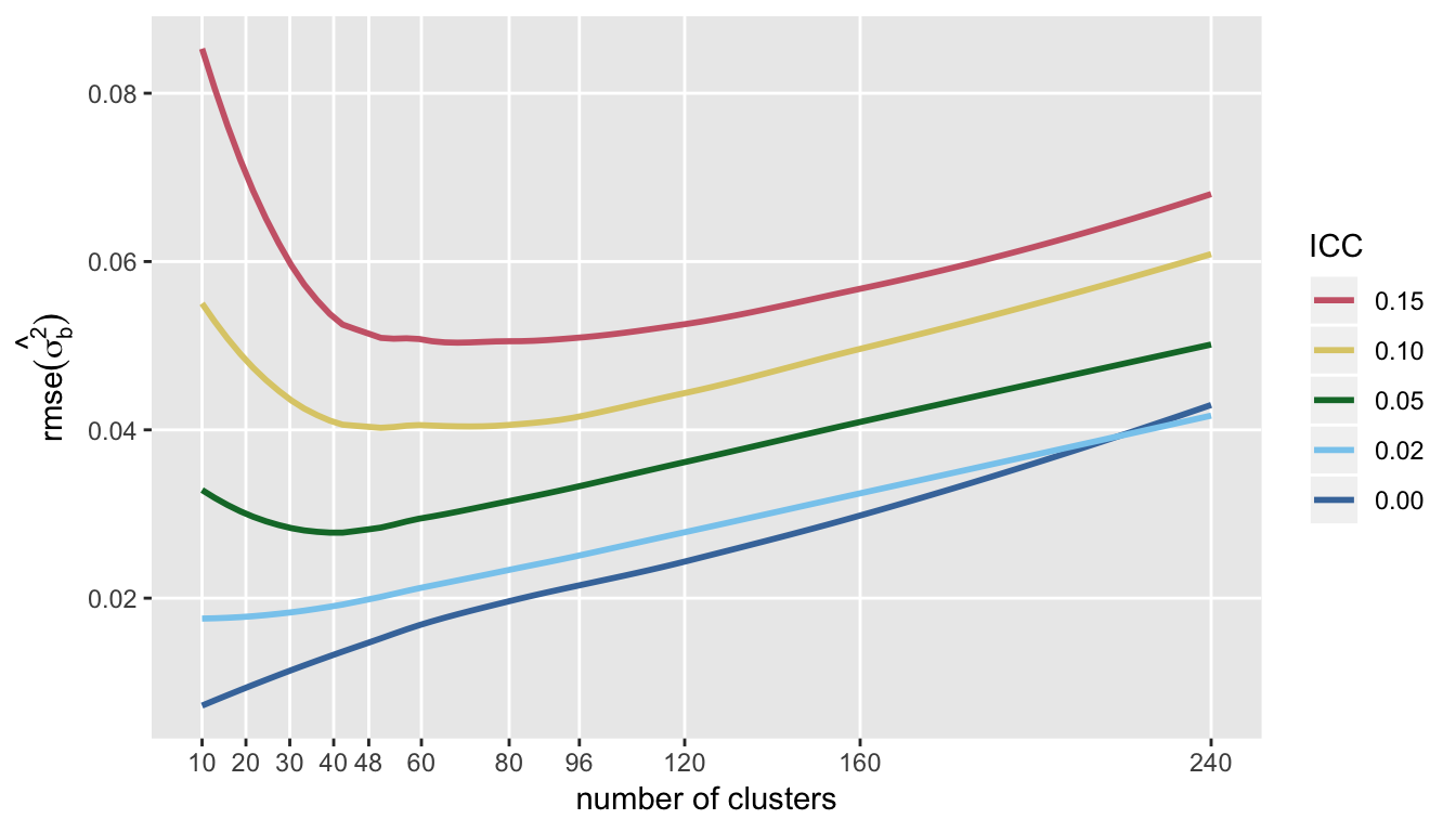
If we are interested in measuring the variation across clusters (which was \(\sigma^2_c\) in the model), then a very different picture emerges. First, the plot of RMSE (which is \(E[(\hat{\theta} - \theta)^2]^{\frac{1}{2}}\), where \(\theta = \sigma^2_c\)), indicates that after some point, actually increasing the number of clusters after a certain point may be a bad idea.
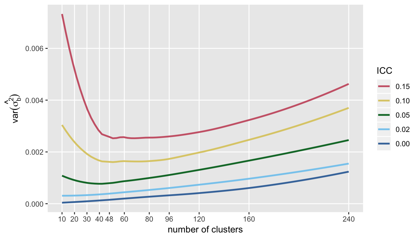
The trends of RMSE are mirrored by the variance of \(\hat{\sigma^2_c}\):
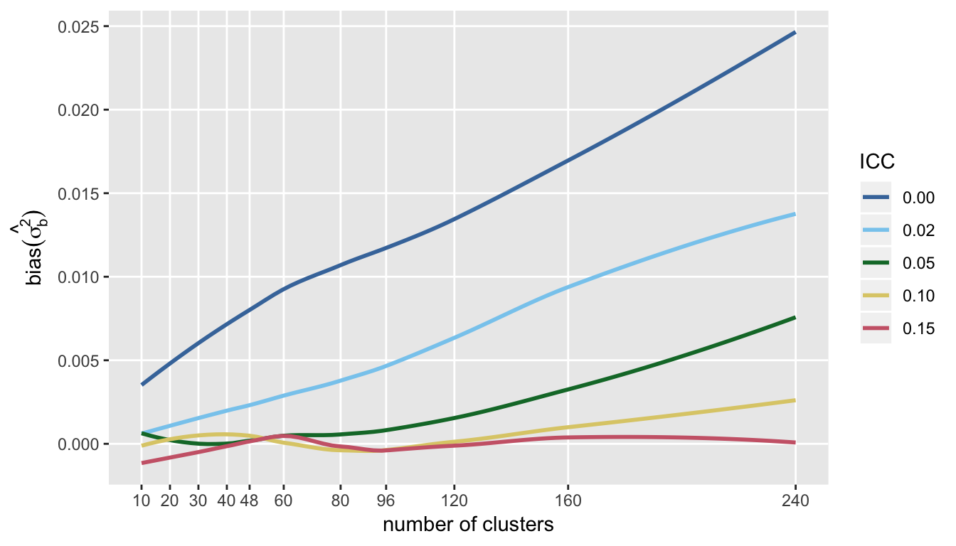
I show the bias of the variance estimate, because it highlights the point that it is very difficult to get an unbiased estimate of \(\sigma^2_c\) when the ICC is low, particularly with a large number of clusters with small cluster sizes. This may not be so surprising, because with small cluster sizes it may be more difficult to estimate the within-cluster variance, an important piece of the total variation.
Almost an addendum
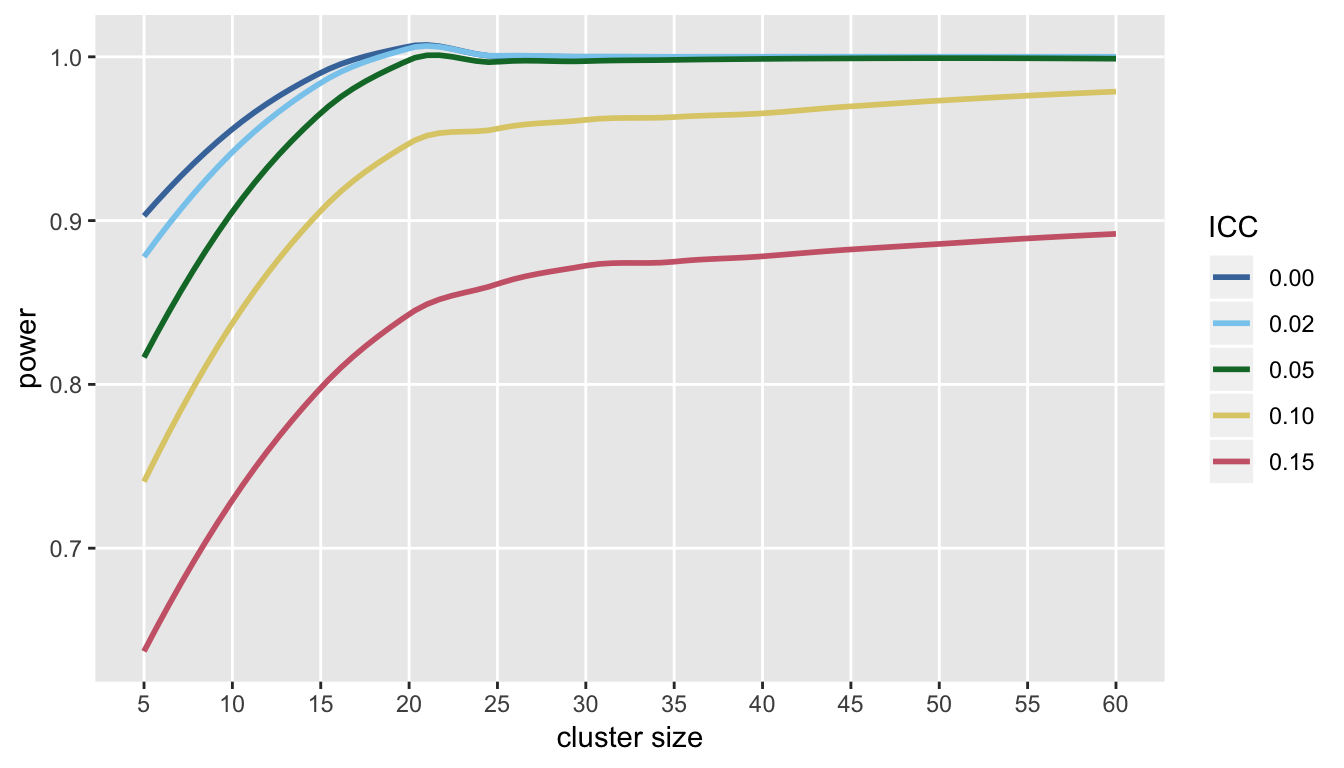
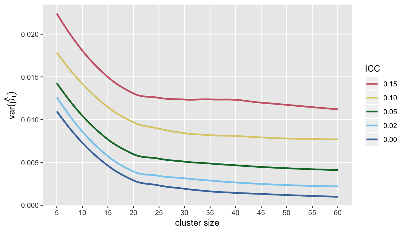
I’ve focused entirely on the direct trade-off between the number of clusters and cluster size, because that was the question raised by the study that motivated this post. However, we may have a fixed number of clusters, and we might want to know if it makes sense to recruit more subjects from each cluster. To get a picture of this, I re-ran the simulations with 60 clusters, by evaluated power and variance of the treatment effect estimator at cluster sizes ranging from 5 to 60.
Under the assumptions used here, it also looks like there is a point after which little can be gained by adding subjects to each cluster (at least in terms of both power and precision of the estimate of the treatment effect):