In a current multi-site study, we are using a stepped-wedge design to evaluate whether improved training and protocols can reduce prescriptions of anti-psychotic medication for home hospice care patients with advanced dementia. The study is officially called the Hospice Advanced Dementia Symptom Management and Quality of Life (HAS-QOL) Stepped Wedge Trial. Unlike my previous work with stepped-wedge designs, where individuals were measured once in the course of the study, this study will collect patient outcomes from the home hospice care EHRs over time. This means that for some patients, the data collection period straddles the transition from control to intervention.
Whenever I contemplate a simulation, I first think about the general structure of the data generating process before even thinking about outcome model. In the case of a more standard two-arm randomized trial, that structure is quite simple and doesn’t require much, if any, thought. In this case, however, the overlaying of a longitudinal patient outcome process on top of a stepped-wedge design presents a little bit of a challenge.
Adding to the challenge is that, in addition to being a function of site- and individual-specific characteristics/effects, the primary outcome will likely be a function of time-varying factors. In particular here, certain patient-level health-related factors that might contribute to the decision to prescribe anti-psychotic medications, and the time-varying intervention status, which is determined by the stepped-wedge randomization scheme. So, the simulation needs to accommodate the generation of both types of time-varying variables.
I’ve developed a bare-boned simulation of sites and patients to provide a structure that I can add to at some point in the future. While this is probably a pretty rare study design (though as stepped-wedge designs become more popular, it may be less rare than I am imagining), I thought the code could provide yet another example of how to approach a potentially vexing simulation in a relatively simple way.
Data definition
The focus here is on the structure of the data, so I am not generating any outcome data. However, in addition to generating the treatment assignment, I am creating the time-varying health status, which will affect the outcome process when I get to that.
In this simulation, there will be 5 sites, each followed for 25 weeks (starting with week 0). Each week, a site will have approximately 20 new patients, so we should expect to generate around \(5 \times 25 \times 20 = 2500\) total patients.
For each patient, we will be generating a series of health status, which ranges from 1 to 4, with 1 being healthiest, and 4 being death. I will use a Markov chain to generate this series. Two arguments required to simulate the Markov process are the starting state (which is created in S0) and the transition matrix P, which determines the probabilities of moving from one state to another.
NPER <- 25
perDef <- defDataAdd(varname = "npatient",  formula = 20,
                     dist = "poisson")

patDef <- defDataAdd(varname = "S0", formula = "0.4;0.4;0.2",
                     dist = "categorical")

P <- t(matrix(c( 0.7, 0.2, 0.1, 0.0,
                 0.1, 0.3, 0.4, 0.2,
                 0.0, 0.1, 0.5, 0.4,
                 0.0, 0.0, 0.0, 1.0),
              nrow = 4))
Data generation
The data generation process starts with the sites and then proceeds to the patient level data. To begin, the five sites are generated (for now without any site-specific variables, but that could easily be modified in the future). Next, records for each site for each of the 25 periods (from week 0 to week 24) are generated; these site level records include the number patients to be generated for each site, each week:
set.seed(3837263)

dsite <- genData(5, id = "site")

dper <- addPeriods(dsite, nPeriods = NPER, idvars = "site",
                   timeid = "site.time", perName = "period")
dper <- addColumns(perDef, dper)

dper
## site period site.time npatient
## 1: 1 0 1 17
## 2: 1 1 2 20
## 3: 1 2 3 25
## 4: 1 3 4 18
## 5: 1 4 5 23
## ---
## 121: 5 20 121 17
## 122: 5 21 122 15
## 123: 5 22 123 16
## 124: 5 23 124 19
## 125: 5 24 125 20Now, we assign each of the five sites to its own intervention “wave”. The first site starts at the beginning of the the study, week 0. The second starts 4 weeks later at week 4, and so on, until the fifth and last site starts the intervention at week 16. (Obviously, a more realistic simulation would include many more sites, but all of this can easily be scaled up.) The intervention indicator is \(I_{ct}\), and is set to 1 when cluster \(c\) during week \(t\) is in the intervention, and is 0 otherwise.
dsw <- trtStepWedge(dper, "site", nWaves = 5, lenWaves = 4,
                    startPer = 0, perName = "period",
                    grpName = "Ict")

dsw <- dsw[, .(site, period, startTrt, Ict)]
Here are the intervention assignments for the first two sites during the first 8 weeks.
dsw[site %in% c(1,2) & period < 8]## site period startTrt Ict
## 1: 1 0 0 1
## 2: 1 1 0 1
## 3: 1 2 0 1
## 4: 1 3 0 1
## 5: 1 4 0 1
## 6: 1 5 0 1
## 7: 1 6 0 1
## 8: 1 7 0 1
## 9: 2 0 4 0
## 10: 2 1 4 0
## 11: 2 2 4 0
## 12: 2 3 4 0
## 13: 2 4 4 1
## 14: 2 5 4 1
## 15: 2 6 4 1
## 16: 2 7 4 1To generate the patients, we start by generating the 2500 or so individual records. The single baseline factor that we include this time around is the starting health status S0.
dpat <- genCluster(dper, cLevelVar = "site.time",
                   numIndsVar = "npatient", level1ID = "id")
dpat <- addColumns(patDef, dpat)
dpat
## site period site.time npatient id S0
## 1: 1 0 1 17 1 2
## 2: 1 0 1 17 2 1
## 3: 1 0 1 17 3 2
## 4: 1 0 1 17 4 2
## 5: 1 0 1 17 5 1
## ---
## 2524: 5 24 125 20 2524 3
## 2525: 5 24 125 20 2525 2
## 2526: 5 24 125 20 2526 1
## 2527: 5 24 125 20 2527 1
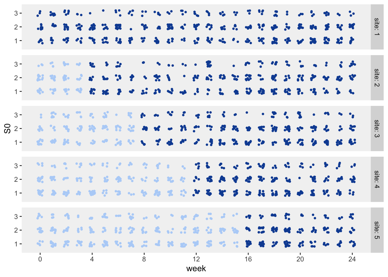
## 2528: 5 24 125 20 2528 1Here is a visualization of the patients (it turns out there are 2528 of them) by site and starting point, with each point representing a patient. The color represents the intervention status: light blue is control (pre-intervention) and dark blue is intervention. Even though a patient may start in the pre-intervention period, they may actually receive services in the intervention period, as we will see further on down.
The patient health status series are generated using a Markov chain process. This particular transition matrix has an “absorbing” state, as indicated by the probability 1 in the last row of the matrix. Once a patient enters state 4, they will not transition to any other state. (In this case, state 4 is death.)
dpat <- addMarkov(dpat, transMat = P,
                  chainLen = NPER, id = "id",
                  pername = "seq", start0lab = "S0")

dpat
## site period site.time npatient id S0 seq state
## 1: 1 0 1 17 1 2 1 2
## 2: 1 0 1 17 1 2 2 3
## 3: 1 0 1 17 1 2 3 3
## 4: 1 0 1 17 1 2 4 3
## 5: 1 0 1 17 1 2 5 4
## ---
## 63196: 5 24 125 20 2528 1 21 4
## 63197: 5 24 125 20 2528 1 22 4
## 63198: 5 24 125 20 2528 1 23 4
## 63199: 5 24 125 20 2528 1 24 4
## 63200: 5 24 125 20 2528 1 25 4Now, we aren’t interested in the periods following the one where death occurs. So, we want to trim the data.table dpat to include only those periods leading up to state 4 and the first period in which state 4 is entered. We do this first by identifying the first time a state of 4 is encountered for each individual (and if an individual never reaches state 4, then all the individual’s records are retained, and the variable .last is set to the maximum number of periods NPER, in this case 25).
dlast <- dpat[, .SD[state == 4][1,], by = id][, .(id, .last = seq)]
dlast[is.na(.last), .last := NPER]

dlast
## id .last
## 1: 1 5
## 2: 2 13
## 3: 3 2
## 4: 4 6
## 5: 5 3
## ---
## 2524: 2524 7
## 2525: 2525 5
## 2526: 2526 19
## 2527: 2527 20
## 2528: 2528 8Next, we use the dlast data.table to “trim” dpat. We further trim the data set so that we do not have patient-level observations that extend beyond the overall follow-up period:
dpat <- dlast[dpat][seq <= .last][ , .last := NULL][]
dpat[, period := period + seq - 1]
dpat <- dpat[period < NPER]

dpat
## id site period site.time npatient S0 seq state
## 1: 1 1 0 1 17 2 1 2
## 2: 1 1 1 1 17 2 2 3
## 3: 1 1 2 1 17 2 3 3
## 4: 1 1 3 1 17 2 4 3
## 5: 1 1 4 1 17 2 5 4
## ---
## 12608: 2524 5 24 125 20 3 1 3
## 12609: 2525 5 24 125 20 2 1 2
## 12610: 2526 5 24 125 20 1 1 1
## 12611: 2527 5 24 125 20 1 1 1
## 12612: 2528 5 24 125 20 1 1 1And finally, we merge the patient data with the stepped-wedge treatment assignment data to create the final data set. The individual outcomes for each week could now be generated, because would we have all the baseline and time-varying information in a single data set.
dpat <- merge(dpat, dsw, by = c("site","period"))
setkey(dpat, id, period)
dpat <- delColumns(dpat, c("site.time", "seq", "npatient"))

dpat
## site period id S0 state startTrt Ict
## 1: 1 0 1 2 2 0 1
## 2: 1 1 1 2 3 0 1
## 3: 1 2 1 2 3 0 1
## 4: 1 3 1 2 3 0 1
## 5: 1 4 1 2 4 0 1
## ---
## 12608: 5 24 2524 3 3 16 1
## 12609: 5 24 2525 2 2 16 1
## 12610: 5 24 2526 1 1 16 1
## 12611: 5 24 2527 1 1 16 1
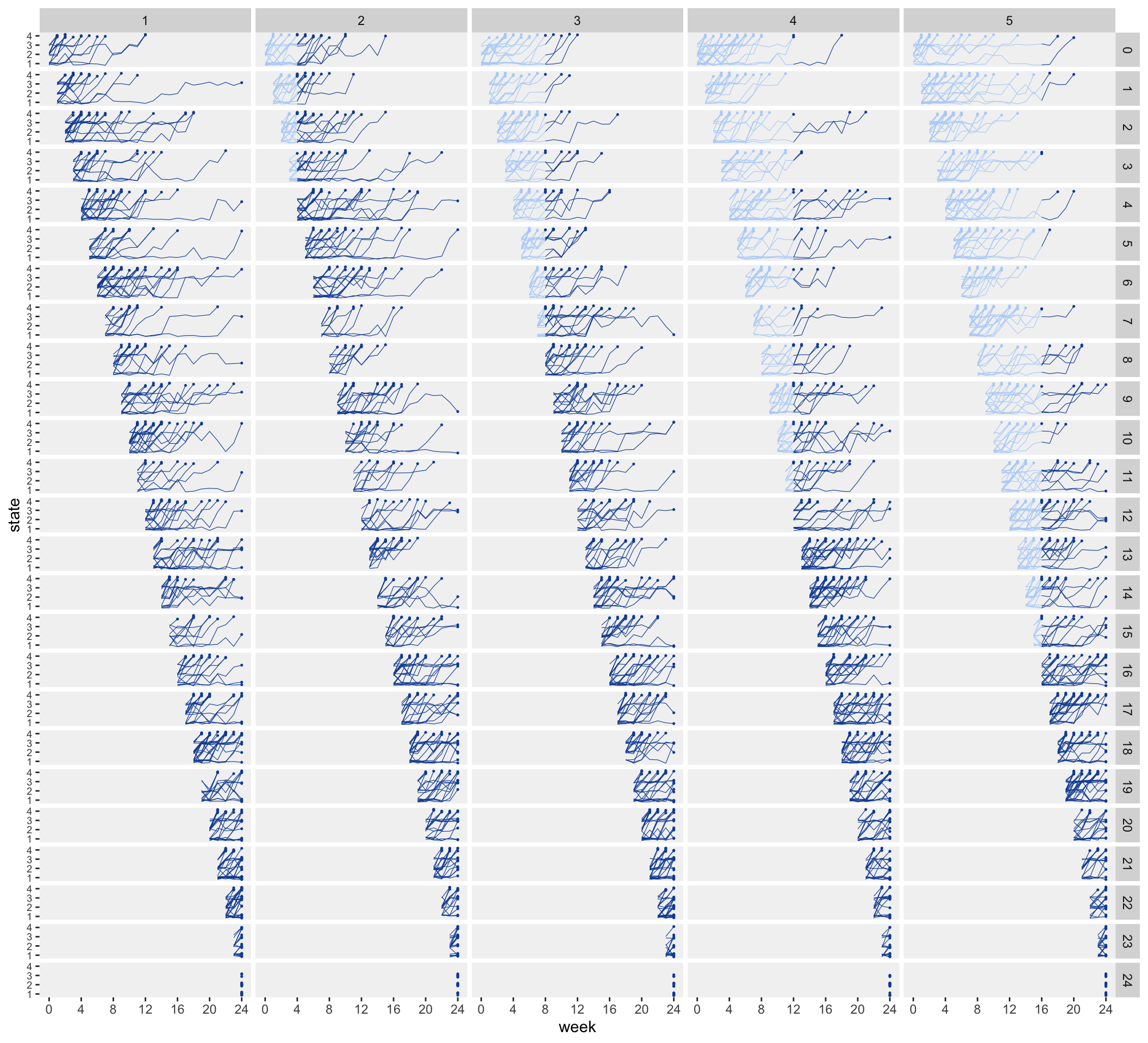
## 12612: 5 24 2528 1 1 16 1Here is what the individual trajectories of health state look like. In the plot, each column represents a different site, and each row represents a different starting week. For example the fifth row represents patients who appear for the first time in week 4. Sites 1 and 2 are already in the intervention in week 4, so none of these patients will transition. However, patients in sites 3 through 5 enter in the pre-intervention stage in week 4, and transition into the intervention at different points, depending on the site.
The basic structure is in place, so we are ready to extend this simulation to include more covariates, random effects, and outcomes. And once we’ve done that, we can explore analytic approaches.
This study is supported by the National Institutes of Health National Institute on Aging R61AG061904. The views expressed are those of the author and do not necessarily represent the official position of the funding organizations.