I learned statistics and probability by simulating data. Sure, I did the occasional proof, but I never believed the results until I saw it in a simulation. I guess I have it backwards, but I that’s just the way I am. And now that I am a so-called professional, I continue to use simulation to understand models, to do sample size estimates and power calculations, and of course to teach. Sure - I’ll use the occasional formula when one exists, but I always feel the need to check it with simulation. It’s just the way I am.
Since I found myself constantly setting up simulations, over time I developed ways to make the process a bit easier. Those processes turned into a package, which I called simstudy, which obviously means simulating study data. The purpose here in this blog entyr is to introduce the basic idea behind simstudy, and provide a relatively brief example that actually comes from a question a user posed about generating correlated longitudinal data.
The basic idea
Simulation using simstudy has two primary steps. First, the user defines the data elements of a data set either in an external csv file or internally through a set of repeated definition statements. Second, the user generates the data, using these definitions. Data generation can be as simple as a cross-sectional design or prospective cohort design, or it can be more involved, extending to allow simulators to generate observed or randomized treatment assignment/exposures, survival data, longitudinal/panel data, multi-level/hierarchical data, datasets with correlated variables based on a specified covariance structure, and to data sets with missing data based on a variety of missingness patterns.
The key to simulating data in simstudy is the creation of series of data defintion tables that look like this:
| varname | formula | variance | dist | link |
|---|---|---|---|---|
| nr | 7 | 0 | nonrandom | identity |
| x1 | 10;20 | 0 | uniform | identity |
| y1 | nr + x1 * 2 | 8 | normal | identity |
| y2 | nr - 0.2 * x1 | 0 | poisson | log |
| xCat | 0.3;0.2;0.5 | 0 | categorical | identity |
| g1 | 5+xCat | 1 | gamma | log |
| a1 | -3 + xCat | 0 | binary | logit |
Here’s the code that is used to generate this definition, which is stored as a data.table :
def <- defData(varname = "nr", dist = "nonrandom", formula=7, id = "idnum")
def <- defData(def,varname="x1",dist="uniform",formula="10;20")
def <- defData(def,varname="y1",formula="nr + x1 * 2",variance=8)
def <- defData(def,varname="y2",dist="poisson",
               formula="nr - 0.2 * x1",link="log")
def <- defData(def,varname="xCat",formula = "0.3;0.2;0.5",dist="categorical")
def <- defData(def,varname="g1", dist="gamma",
               formula = "5+xCat", variance = 1, link = "log")
def <- defData(def, varname = "a1", dist = "binary" ,
               formula="-3 + xCat", link="logit")
To create a simple data set based on these definitions, all one needs to do is execute a single genData command. In this example, we generate 500 records that are based on the definition in the deftable:
dt <- genData(500, def)

dt
## idnum nr x1 y1 y2 xCat g1 a1
## 1: 1 7 19.41283 47.02270 17 2 2916.191027 0
## 2: 2 7 17.93997 44.71866 29 1 2015.266701 0
## 3: 3 7 17.53885 43.96838 31 3 775.414175 0
## 4: 4 7 14.39268 37.89804 67 1 6.478367 0
## 5: 5 7 11.08339 30.20787 120 3 1790.472665 1
## ---
## 496: 496 7 15.57788 34.36490 45 3 13016.890610 1
## 497: 497 7 11.06041 26.95209 132 1 592.113025 0
## 498: 498 7 18.49925 46.86620 25 1 84.521499 0
## 499: 499 7 11.89009 33.60175 87 3 4947.826967 1
## 500: 500 7 18.70241 44.96824 33 2 695.362237 0There’s a lot more functionality in the package, and I’ll be writing about that in the future. But here, I just want give a little more introduction by way of an example that came in from around the world a couple of days ago. (I’d say the best thing about building a package is hearing from folks literally all over the world and getting to talk to them about statistics and R. It is really incredible to be able to do that.)
Going a bit further: simulating a prosepctive cohort study with repeated measures
The question was, can we simulate a study with two arms, say a control and treatment, with repeated measures at three time points: baseline, after 1 month, and after 2 months? Of course.
This was what I sent back to my correspondent:
# Define the outcome

ydef <- defDataAdd(varname = "Y", dist = "normal",
                   formula = "5 + 2.5*period + 1.5*T + 3.5*period*T",
                   variance = 3)

# Generate a "blank" data.table with 24 observations and
# assign them to groups

set.seed(1234)

indData <- genData(24)
indData <- trtAssign(indData, nTrt = 2, balanced = TRUE, grpName = "T")

# Create a longitudinal data set of 3 records for each id

longData <- addPeriods(indData, nPeriods = 3, idvars = "id")
longData <- addColumns(dtDefs = ydef, longData)

longData[, T := factor(T, labels = c("No", "Yes"))]

# Let's look at the data

ggplot(data = longData, aes(x = factor(period), y = Y)) +
  geom_line(aes(color = T, group = id)) +
  scale_color_manual(values = c("#e38e17", "#8e17e3")) +
  xlab("Time")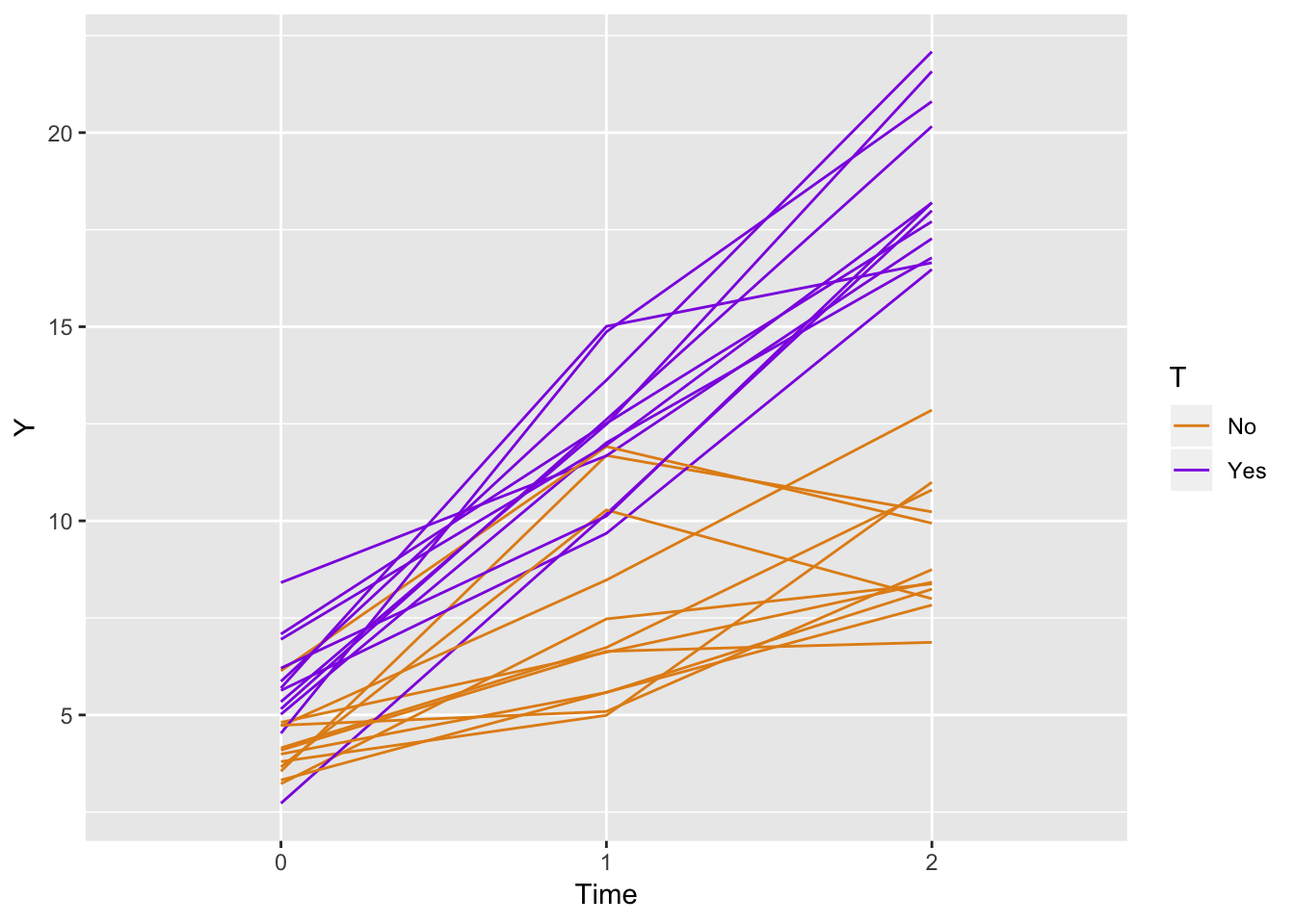
If we generate a data set based on 1,000 indviduals and estimate a linear regression model we see that the parameter estimates are quite good. However, my correspondent wrote back saying she wanted correlated data, which makes sense. We can see from the alpha estimate of approximately 0.02 (at the bottom of the output), we don’t have much correlation:
# Fit a GEE model to the data

fit <- geeglm(Y~factor(T)+period+factor(T)*period,
              family= gaussian(link= "identity"),
              data=longData, id=id, corstr = "exchangeable")
summary(fit)
##
## Call:
## geeglm(formula = Y ~ factor(T) + period + factor(T) * period,
## family = gaussian(link = "identity"), data = longData, id = id,
## corstr = "exchangeable")
##
## Coefficients:
## Estimate Std.err Wald Pr(>|W|)
## (Intercept) 4.98268 0.07227 4753.4 <2e-16 ***
## factor(T)Yes 1.48555 0.10059 218.1 <2e-16 ***
## period 2.53946 0.05257 2333.7 <2e-16 ***
## factor(T)Yes:period 3.51294 0.07673 2096.2 <2e-16 ***
## ---
## Signif. codes: 0 '***' 0.001 '**' 0.01 '*' 0.05 '.' 0.1 ' ' 1
##
## Estimated Scale Parameters:
## Estimate Std.err
## (Intercept) 2.952 0.07325
##
## Correlation: Structure = exchangeable Link = identity
##
## Estimated Correlation Parameters:
## Estimate Std.err
## alpha 0.01737 0.01862
## Number of clusters: 1000 Maximum cluster size: 3One way to generate correlated data
The first way to approach this is to use the simstudy function genCorData to generate correlated errors that are normally distributed with mean 0, variance of 3, and and common correlation coeffcient of 0.7. This approach is a bit mysterious, because we are acknowledging that we don’t know what is driving the relationship between the three outcomes, just that they have a common cause.
# define the outcome
ydef <- defDataAdd(varname = "Y", dist = "normal",
            formula = "5 + 2.5*period + 1.5*T + 3.5*period*T + e")

# define the correlated errors

mu <- c(0, 0, 0)
sigma <- rep(sqrt(3), 3)

# generate correlated data for each id and assign treatment

dtCor <- genCorData(24, mu = mu, sigma = sigma, rho = .7, corstr = "cs")
dtCor <- trtAssign(dtCor, nTrt = 2, balanced = TRUE, grpName = "T")

# create longitudinal data set and generate outcome based on definition

longData <- addPeriods(dtCor, nPeriods = 3, idvars = "id", timevars = c("V1","V2", "V3"), timevarName = "e")
longData <- addColumns(ydef, longData)

longData[, T := factor(T, labels = c("No", "Yes"))]

# look at the data, outcomes should appear more correlated,
# lines a bit straighter

ggplot(data = longData, aes(x = factor(period), y = Y)) +
  geom_line(aes(color = T, group = id)) +
  scale_color_manual(values = c("#e38e17", "#8e17e3")) +
  xlab("Time")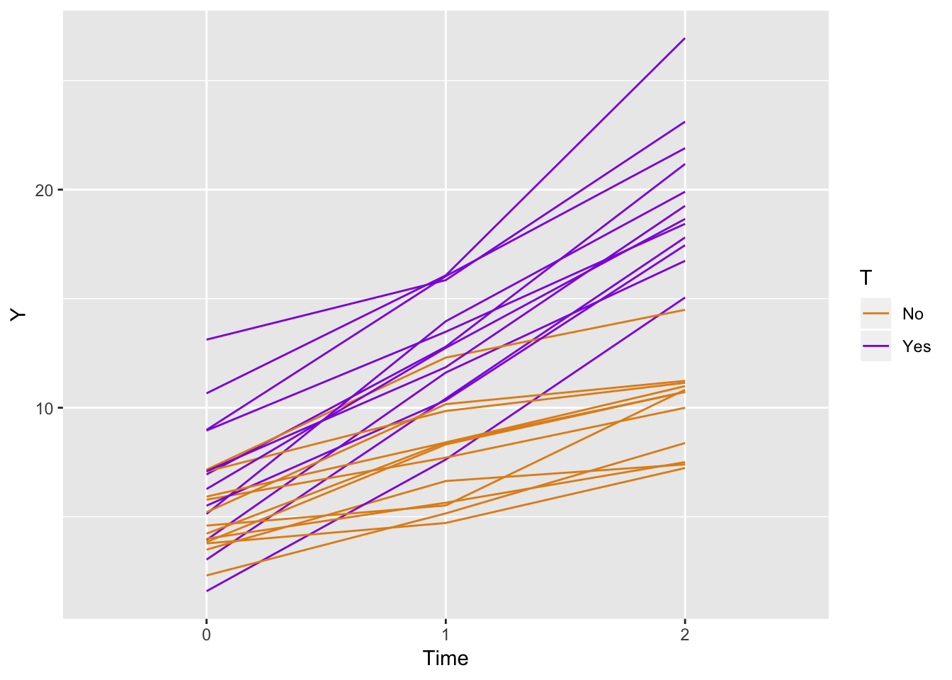
Again, we recover the true parameters. And this time, if we look at the estimated correlation, we see that indeed the outcomes are correlated within each indivdual. The estimate is 0.77, close to the our specified value of 0.7.
fit <- geeglm(Y~factor(T)+period+factor(T)*period,
              family = gaussian(link= "identity"),
              data = longData, id = id, corstr = "exchangeable")

summary(fit)
##
## Call:
## geeglm(formula = Y ~ factor(T) + period + factor(T) * period,
## family = gaussian(link = "identity"), data = longData, id = id,
## corstr = "exchangeable")
##
## Coefficients:
## Estimate Std.err Wald Pr(>|W|)
## (Intercept) 5.0700 0.0770 4335 <2e-16 ***
## factor(T)Yes 1.5693 0.1073 214 <2e-16 ***
## period 2.4707 0.0303 6670 <2e-16 ***
## factor(T)Yes:period 3.5379 0.0432 6717 <2e-16 ***
## ---
## Signif. codes: 0 '***' 0.001 '**' 0.01 '*' 0.05 '.' 0.1 ' ' 1
##
## Estimated Scale Parameters:
## Estimate Std.err
## (Intercept) 3.01 0.107
##
## Correlation: Structure = exchangeable Link = identity
##
## Estimated Correlation Parameters:
## Estimate Std.err
## alpha 0.702 0.0135
## Number of clusters: 1000 Maximum cluster size: 3Another way to generate correlated data
A second way to generate correlatd data is through an individual level random-effect or random intercept. This could be considered some unmeasured characteristic of the individuals (which happens to have a convenient normal distribution with mean zero). This random effect contributes equally to all instances of an individuals outcomes, but the outcomes for a particular individual deviate slightly from the hypothetical straight line as a result of unmeasured noise.
ydef1 <- defData(varname = "randomEffect", dist = "normal",
                 formula = 0, variance = sqrt(3))

ydef2 <- defDataAdd(varname = "Y", dist = "normal",
    formula = "5 + 2.5*period + 1.5*T + 3.5*period*T + randomEffect",
    variance = 1)

indData <- genData(24, ydef1)
indData <- trtAssign(indData, nTrt = 2, balanced = TRUE, grpName = "T")

indData[1:6]
## id T randomEffect
## 1: 1 0 -1.3101
## 2: 2 1 0.3423
## 3: 3 0 0.5716
## 4: 4 1 2.6723
## 5: 5 0 -0.9996
## 6: 6 1 -0.0722longData <- addPeriods(indData, nPeriods = 3, idvars = "id")
longData <- addColumns(dtDefs = ydef2, longData)
longData[, T := factor(T, labels = c("No", "Yes"))]
ggplot(data = longData, aes(x = factor(period), y = Y)) +
geom_line(aes(color = T, group = id)) +
scale_color_manual(values = c("#e38e17", "#8e17e3")) +
xlab("Time")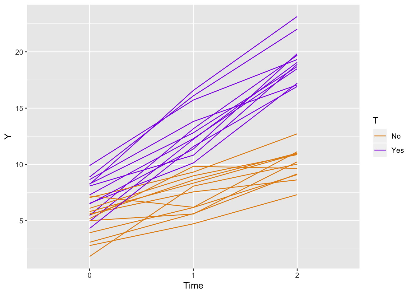
fit <- geeglm(Y~factor(T)+period+factor(T)*period,
              family= gaussian(link= "identity"),
              data = longData, id = id, corstr = "exchangeable")
summary(fit)
##
## Call:
## geeglm(formula = Y ~ factor(T) + period + factor(T) * period,
## family = gaussian(link = "identity"), data = longData, id = id,
## corstr = "exchangeable")
##
## Coefficients:
## Estimate Std.err Wald Pr(>|W|)
## (Intercept) 4.9230 0.0694 5028 <2e-16 ***
## factor(T)Yes 1.4848 0.1003 219 <2e-16 ***
## period 2.5310 0.0307 6793 <2e-16 ***
## factor(T)Yes:period 3.5076 0.0449 6104 <2e-16 ***
## ---
## Signif. codes: 0 '***' 0.001 '**' 0.01 '*' 0.05 '.' 0.1 ' ' 1
##
## Estimated Scale Parameters:
## Estimate Std.err
## (Intercept) 2.63 0.0848
##
## Correlation: Structure = exchangeable Link = identity
##
## Estimated Correlation Parameters:
## Estimate Std.err
## alpha 0.619 0.0146
## Number of clusters: 1000 Maximum cluster size: 3I sent all this back to my correspondent, but I haven’t heard yet if it is what she wanted. I certainly hope so. If there are specific topics you’d like me to discuss related to simstudy, definitely get in touch, and I will try to write something up.