I’ve been working on updates for the simstudy package. In the past few weeks, a couple of folks independently reached out to me about generating correlated binary data. One user was not impressed by the copula algorithm that is already implemented. I’ve added an option to use an algorithm developed by Emrich and Piedmonte in 1991, and will be incorporating that option soon in the functions genCorGen and addCorGen. I’ll write about that change some point soon.
A second researcher was trying to generate data using parameters that could be recovered using GEE model estimation. I’ve always done this by using an underlying mixed effects model, but of course, the marginal model parameter estimates might be quite different from the conditional parameters. (I’ve written about this a number of times, most recently here.) As a result, the model and the data generation process don’t match, which may not be such a big deal, but is not so helpful when trying to illuminate the models.
One simple solution is using a beta-binomial mixture data generating process. The beta distribution is a continuous probability distribution that is defined on the interval from 0 to 1, so it is not too unreasonable as model for probabilities. If we assume that cluster-level probabilities have a beta distribution, and that within each cluster the individual outcomes have a binomial distribution defined by the cluster-specific probability, we will get the data generation process we are looking for.
Generating the clustered data
In these examples, I am using 500 clusters, each with cluster size of 40 individuals. There is a cluster-level covariate x that takes on integer values between 1 and 3. The beta distribution is typically defined using two shape parameters usually referenced as \(\alpha\) and \(\beta,\) where \(E(Y) = \alpha / (\alpha + \beta),\) and \(Var(Y) = (\alpha\beta)/[(\alpha + \beta)^2(\alpha + \beta + 1)].\) In simstudy, the distribution is specified using the mean probability, \(p_m,\) and a precision parameter, \(\phi_\beta > 0,\) which is specified using the variance argument. Under this specification, \(Var(Y) = p_m(1 - p_m)/(1 + \phi_\beta).\) Precision is inversely related to variability: lower precision is higher variability.
In this simple simulation, the cluster probabilities are a function of the cluster-level covariate and precision parameter \(\phi_\beta\). Specifically
\[logodds(p_{clust}) = -2.0 + 0.65x.\] The binomial variable of interest \(b\) is a function of \(p_{clust}\) only, and represents a count of individuals in the cluster with a “success”:
library(simstudy)

set.seed(87387)

phi.beta <- 3       # precision
n <- 40             # cluster size

def <- defData(varname = "n", formula = n,
               dist = 'nonrandom', id = "cID")
def <- defData(def, varname = "x", formula = "1;3",
               dist = 'uniformInt')
def <- defData(def, varname = "p", formula = "-2.0 + 0.65 * x",
               variance = phi.beta, dist = "beta", link = "logit")
def <- defData(def, varname = "b", formula = "p", variance = n,
               dist = "binomial")

dc <- genData(500, def)
dc
## cID n x p b
## 1: 1 40 2 0.101696930 4
## 2: 2 40 2 0.713156596 32
## 3: 3 40 1 0.020676443 2
## 4: 4 40 2 0.091444678 4
## 5: 5 40 2 0.139946091 6
## ---
## 496: 496 40 1 0.062513419 4
## 497: 497 40 1 0.223149651 5
## 498: 498 40 3 0.452904009 14
## 499: 499 40 2 0.005143594 1
## 500: 500 40 2 0.481283809 16The generated data with \(\phi_\beta = 3\) is shown on the left below. Data sets with increasing precision (less variability) are shown to the right:
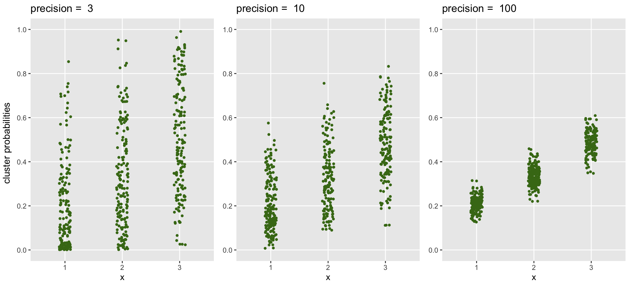
The relationship of \(\phi_\beta\) and variance is made clear by evaluating the variance of the cluster probabilities at each level of \(x\) and comparing these variance estimates with the theoretical values suggested by parameters specified in the data generation process:
p.clust = 1/(1 + exp(2 - 0.65*(1:3)))

cbind(dc[, .(obs = round(var(p), 3)), keyby = x],
    theory = round( (p.clust*(1 - p.clust))/(1 + phi.beta), 3))
## x obs theory
## 1: 1 0.041 0.041
## 2: 2 0.054 0.055
## 3: 3 0.061 0.062Beta and beta-binomial regression
Before getting to the GEE estimation, here are two less frequently used regression models: beta and beta-binomial regression. Beta regression may not be super-useful, because we would need to observe (and measure) the probabilities directly. In this case, we randomly generated the probabilities, so it is fair to estimate a regression model to recover the same parameters we used to generate the data! But, back in the real world, we might only observe \(\hat{p}\), which results from generating data based on the underlying true \(p\). This is where we will need the beta-binomial regression (and later, the GEE model).
First, here is the beta regression using package betareg, which provides quite good estimates of the two coefficients and the precision parameter \(\phi_\beta\), which is not so surprising given the large number of clusters in our sample:
library(betareg)
model.beta <- betareg(p ~ x, data = dc, link = "logit")
summary(model.beta)
##
## Call:
## betareg(formula = p ~ x, data = dc, link = "logit")
##
## Standardized weighted residuals 2:
## Min 1Q Median 3Q Max
## -3.7420 -0.6070 0.0306 0.6699 3.4952
##
## Coefficients (mean model with logit link):
## Estimate Std. Error z value Pr(>|z|)
## (Intercept) -2.09663 0.12643 -16.58 <2e-16 ***
## x 0.70080 0.05646 12.41 <2e-16 ***
##
## Phi coefficients (precision model with identity link):
## Estimate Std. Error z value Pr(>|z|)
## (phi) 3.0805 0.1795 17.16 <2e-16 ***
## ---
## Signif. codes: 0 '***' 0.001 '**' 0.01 '*' 0.05 '.' 0.1 ' ' 1
##
## Type of estimator: ML (maximum likelihood)
## Log-likelihood: 155.2 on 3 Df
## Pseudo R-squared: 0.2388
## Number of iterations: 13 (BFGS) + 1 (Fisher scoring)The beta-binomial regression model, which is estimated using package aod, is a reasonable model to fit in this case where we have observed binomial outcomes and unobserved underlying probabilities:
library(aod)
model.betabinom <- betabin(cbind(b, n - b) ~ x, ~ 1, data = dc)
model.betabinom
## Beta-binomial model
## -------------------
## betabin(formula = cbind(b, n - b) ~ x, random = ~1, data = dc)
##
## Convergence was obtained after 100 iterations.
##
## Fixed-effect coefficients:
## Estimate Std. Error z value Pr(> |z|)
## (Intercept) -2.103e+00 1.361e-01 -1.546e+01 0e+00
## x 6.897e-01 6.024e-02 1.145e+01 0e+00
##
## Overdispersion coefficients:
## Estimate Std. Error z value Pr(> z)
## phi.(Intercept) 2.412e-01 1.236e-02 1.951e+01 0e+00
##
## Log-likelihood statistics
## Log-lik nbpar df res. Deviance AIC AICc
## -1.711e+03 3 497 1.752e+03 3.428e+03 3.428e+03A couple of interesting things to note here. First is that the coefficient estimates are pretty similar to the beta regression model. However, the standard errors are slightly higher, as they should be, since we are using only observed probabilities and not the true (albeit randomly selected or generated) probabilities. So, there is another level of uncertainty beyond sampling error.
Second, there is a new parameter: \(\phi_{overdisp}\). What is that, and how does that relate to \(\phi_\beta\)? The variance of a binomial random variable \(Y\) with a single underlying probability is \(Var(Y) = np(1-p)\). However, when the underlying probability varies across different subgroups (or clusters), the variance is augmented by \(\phi_{overdisp}\): \(Var(Y) = np(1-p)[1 + (n-1)\phi_{overdisp}]\). It turns out to be the case that \(\phi_{overdisp} = 1/(1+\phi_\beta)\):
round(model.betabinom@random.param, 3) # from the beta - binomial model## phi.(Intercept)
## 0.241round(1/(1 + coef(model.beta)["(phi)"]), 3) # from the beta model## (phi)
## 0.245The observed variances of the binomial outcome \(b\) at each level of \(x\) come quite close to the theoretical variances based on \(\phi_\beta\):
phi.overdisp <- 1/(1+phi.beta)

cbind(dc[, .(obs = round(var(b),1)), keyby = x],
  theory = round( n*p.clust*(1-p.clust)*(1 + (n-1)*phi.overdisp), 1))
## x obs theory
## 1: 1 69.6 70.3
## 2: 2 90.4 95.3
## 3: 3 105.2 107.4GEE and individual level data
With individual level binary outcomes (as opposed to count data we were working with before), GEE models are appropriate. The code below generates individual-level for each cluster level:
defI <- defDataAdd(varname = "y", formula = "p", dist = "binary")

di <- genCluster(dc, "cID", numIndsVar = "n", level1ID = "id")
di <- addColumns(defI, di)
di
## cID n x p b id y
## 1: 1 40 2 0.1016969 4 1 0
## 2: 1 40 2 0.1016969 4 2 0
## 3: 1 40 2 0.1016969 4 3 0
## 4: 1 40 2 0.1016969 4 4 0
## 5: 1 40 2 0.1016969 4 5 0
## ---
## 19996: 500 40 2 0.4812838 16 19996 1
## 19997: 500 40 2 0.4812838 16 19997 0
## 19998: 500 40 2 0.4812838 16 19998 1
## 19999: 500 40 2 0.4812838 16 19999 1
## 20000: 500 40 2 0.4812838 16 20000 0The GEE model provides estimates of the coefficients as well as the working correlation. If we assume an “exchangeable” correlation matrix, in which each individual is correlated with all other individuals in the cluster but is not correlated with individuals in other clusters, we will get a single correlation estimate, which is labeled as alpha in the GEE output:
library(geepack)

geefit <- geeglm(y ~ x, family = "binomial", data = di,
                 id = cID, corstr = "exchangeable" )
summary(geefit)
##
## Call:
## geeglm(formula = y ~ x, family = "binomial", data = di, id = cID,
## corstr = "exchangeable")
##
## Coefficients:
## Estimate Std.err Wald Pr(>|W|)
## (Intercept) -2.05407 0.14854 191.2 <2e-16 ***
## x 0.68965 0.06496 112.7 <2e-16 ***
## ---
## Signif. codes: 0 '***' 0.001 '**' 0.01 '*' 0.05 '.' 0.1 ' ' 1
##
## Correlation structure = exchangeable
## Estimated Scale Parameters:
##
## Estimate Std.err
## (Intercept) 1.001 0.03192
## Link = identity
##
## Estimated Correlation Parameters:
## Estimate Std.err
## alpha 0.2493 0.01747
## Number of clusters: 500 Maximum cluster size: 40In this case, alpha (\(\alpha\)) is estimated at 0.25, which is quite close to the previous estimate of \(\phi_{overdisp}\), 0.24. So, it appears to be the case that if we have a target correlation \(\alpha\), we know the corresponding \(\phi_\beta\) to use in the beta-binomial data generation process. That is, \(\phi_\beta = (1 - \alpha)/\alpha\).
While this is certainly not a proof of anything, let’s give it a go with a target \(\alpha = 0.44\):
phi.beta.new <- (1-0.44)/0.44
def <- updateDef(def, "p", newvariance = phi.beta.new)

dc2 <- genData(500, def)
di2 <- genCluster(dc2, "cID", numIndsVar = "n", level1ID = "id")
di2 <- addColumns(defI, di2)

geefit <- geeglm(y ~ x, family = "binomial", data = di2,
                 id = cID, corstr = "exchangeable" )
summary(geefit)
##
## Call:
## geeglm(formula = y ~ x, family = "binomial", data = di2, id = cID,
## corstr = "exchangeable")
##
## Coefficients:
## Estimate Std.err Wald Pr(>|W|)
## (Intercept) -2.0472 0.1844 123.2 <2e-16 ***
## x 0.6994 0.0804 75.6 <2e-16 ***
## ---
## Signif. codes: 0 '***' 0.001 '**' 0.01 '*' 0.05 '.' 0.1 ' ' 1
##
## Correlation structure = exchangeable
## Estimated Scale Parameters:
##
## Estimate Std.err
## (Intercept) 1 0.0417
## Link = identity
##
## Estimated Correlation Parameters:
## Estimate Std.err
## alpha 0.44 0.0276
## Number of clusters: 500 Maximum cluster size: 40Addendum
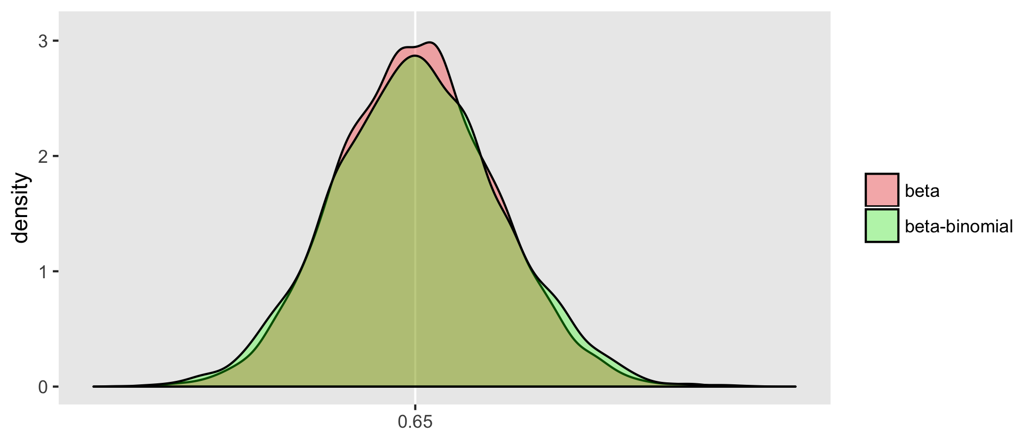
Above, I suggested that the estimator of the effect of x based on the beta model will have less variation than the estimator based on the beta-binomial model. I drew 5000 samples from the data generating process and estimated the models each time. Below is a density distribution of the estimates of each of the models from all 5000 iterations. As expected, the beta-binomial process has more variability, as do the related estimates; we can see this in the relative “peakedness”" of the beta density:
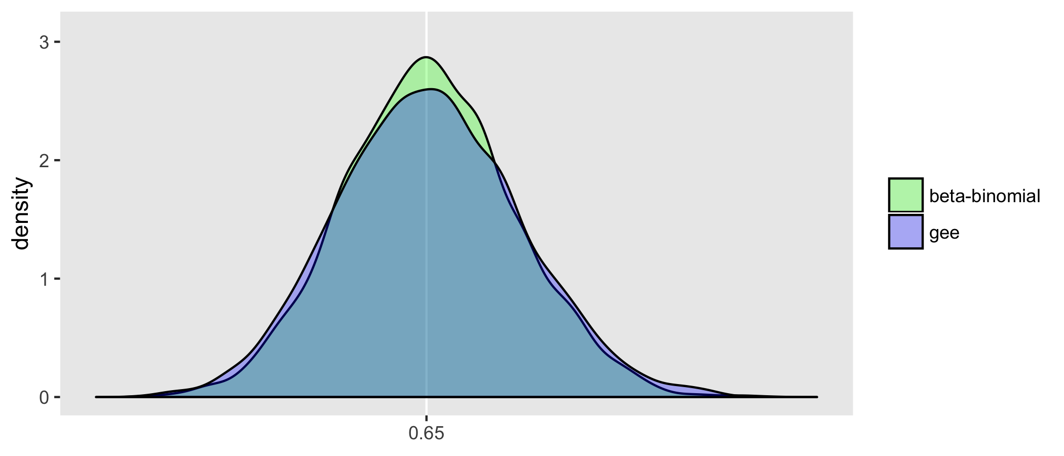
Also based on these 5000 iterations, the GEE model estimation appears to be less efficient than the beta-binomial model. This is not surprising since the beta-binomial model was the actual process that generated the data (so it is truly the correct model). The GEE model is robust to mis-specification of the correlation structure, but the price we pay for that robustness is a slightly less precise estimate (even if we happen to get the correlation structure right):